## Read the complete lecture
Can a few candies held in my fist speak for the whole candy box? Using the candy-drawing metaphor, we distinguish descriptive statistics, which summarizes the drawn candies as they are, from inferential statistics, which estimates the whole box from their pattern.
The Week 10 lecture for the graduate course Communication Research Methods II at Hallym University Media School. The two sets of Week 5 materials from the 2024 undergraduate research methods course were merged into one and rebuilt with Achmage Presentation, keeping their wording and order unchanged. It covers population and sample; the mode · median · mean; variance and standard deviation; the normal distribution and the trap of the mean; and the confidence interval obtained with t.test.
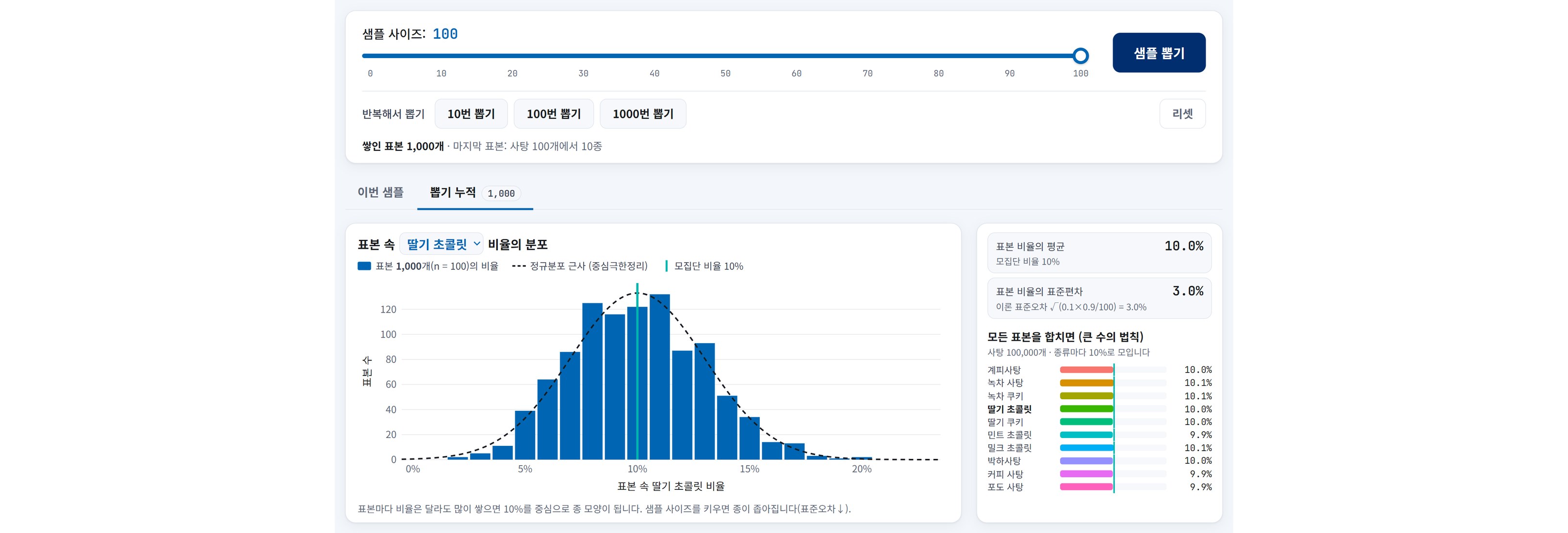
The R code on the slides is shown together with the results of actually running it in R 4.3.3, and the results on the exercise slides appear on the next click. The candy-drawing simulator slide links to a page that ports the R Shiny code to the web, where you can stack up samples 10 · 100 · 1000 times and watch the sample proportions gather in a bell shape around the population proportion. The concept diagrams were drawn with Achmage Pele, and the photos and illustrations are originals from the 2024 lecture materials (original sources not stated).
Includes the Korean slides and full reading version, with English introduction and reading.
## 01\. 10W-1
Communication Research Methods II (Fall 2026)
### Supporting text from the original screen
01 / 77
10W-1 · 1/1
## 02\. Population and sample – a Halloween random candy and chocolate box

Photo of a Halloween candy box full of candies and chocolates
### Supporting text from the original screen
02 / 77
Population and sample · 1/5
## 03\. Let us grab some candy with our fists.
**Population**
The method does not matter. What are the exact proportions of the candies in the whole box?
**Shall we grab just a few?**
Sample 1
**OR · Shall we grab a fistful so full it bursts?**
Sample 2

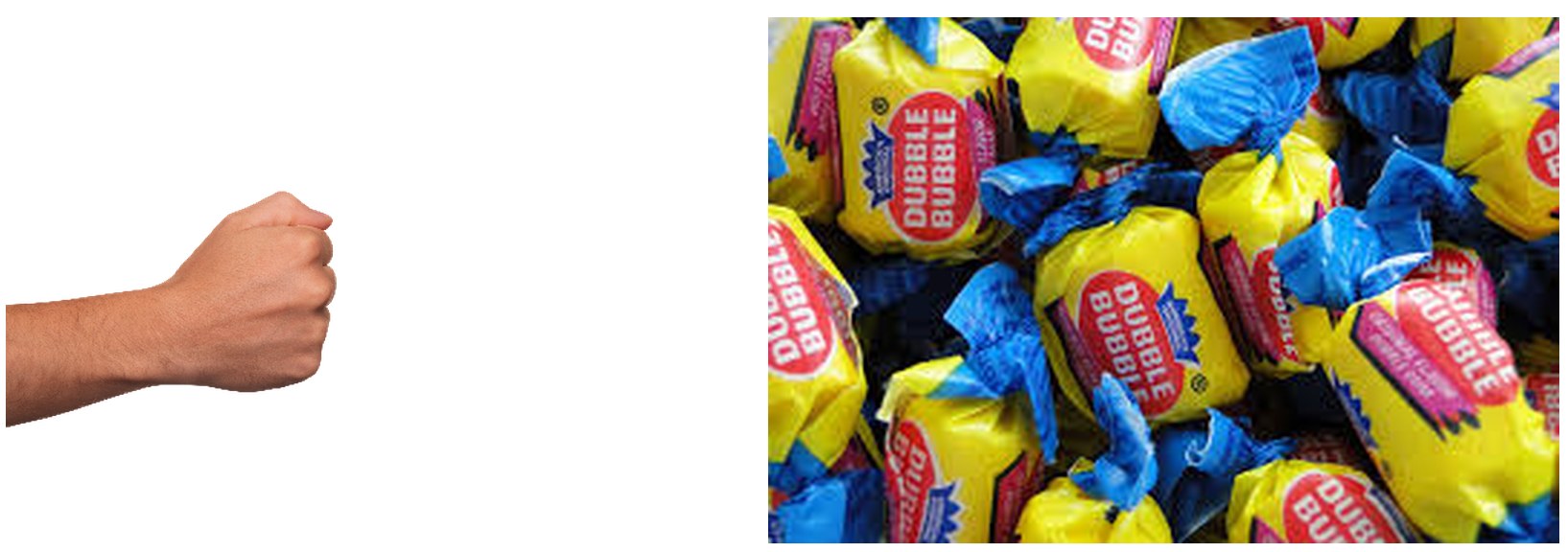
Photos, from left: a box full of candy (population), a fist and only a few candies (Sample 1), and a fist and a big pile of bubble gum (Sample 2)
### Supporting text from the original screen
03 / 77
Population and sample · 2/5
## 04\. Let us grab some candy with our fists.
**Population**
Candy box – the entire population of Korea
**Shall we grab just a few?**
Sample 1 – survey of 1,000 people
**OR · Shall we grab a fistful so full it bursts?**
Sample 2 – survey of 100,000 people

Photos, from left: a box full of candy (population), a fist and only a few candies (Sample 1), and a fist and a big pile of bubble gum (Sample 2)
### Supporting text from the original screen
04 / 77
Population and sample · 3/5
## 05\. Population and sample
* Population: the entire group the researcher wants to know about (e.g., “the entire population of Korea”)
* Sample: a subset of the population that the researcher can observe and that carries the population's characteristics (e.g., “Since I cannot know the entire population of Korea… one by one, I picked only 1000 people out of the entire population of Korea… - a sample of 1000”)
* I am not a tycoon, so I cannot survey everyone in Korea (a census of the population is impossible)
* With a mere few million won, I can survey about 1000–2000 people (drawing a sample according to the research purpose)
* What makes it possible to estimate the entire population of Korea from the data of those 1000–2000 people I collected is none other than statistics (estimating the population through a sample)
### Supporting text from the original screen
05 / 77
Population and sample · 4/5
## 06\. Descriptive statistics and inferential statistics

Inside the outer box “Population: the entire population of Korea” is “A population within the population: Korea's entire tennis-playing population”. An arrow goes from the tennis-playing population to “A sample of the population within the population: the sample of tennis players I picked to represent Korea's entire tennis-playing population..”. From the sample, the flow leads to “Analyzing the characteristics of the sample” (descriptive statistics: the features of the tennis-player sample I picked), then through “Judging whether to generalize” to “Estimating the characteristics of the whole population” (inferential statistics: whether tennis players will influence the image of Korean tennis), and the last arrow returns to the population.
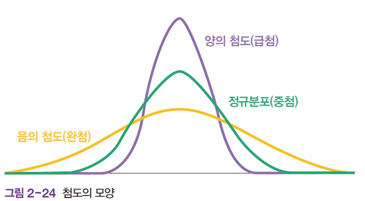
### Supporting text from the original screen
06 / 77
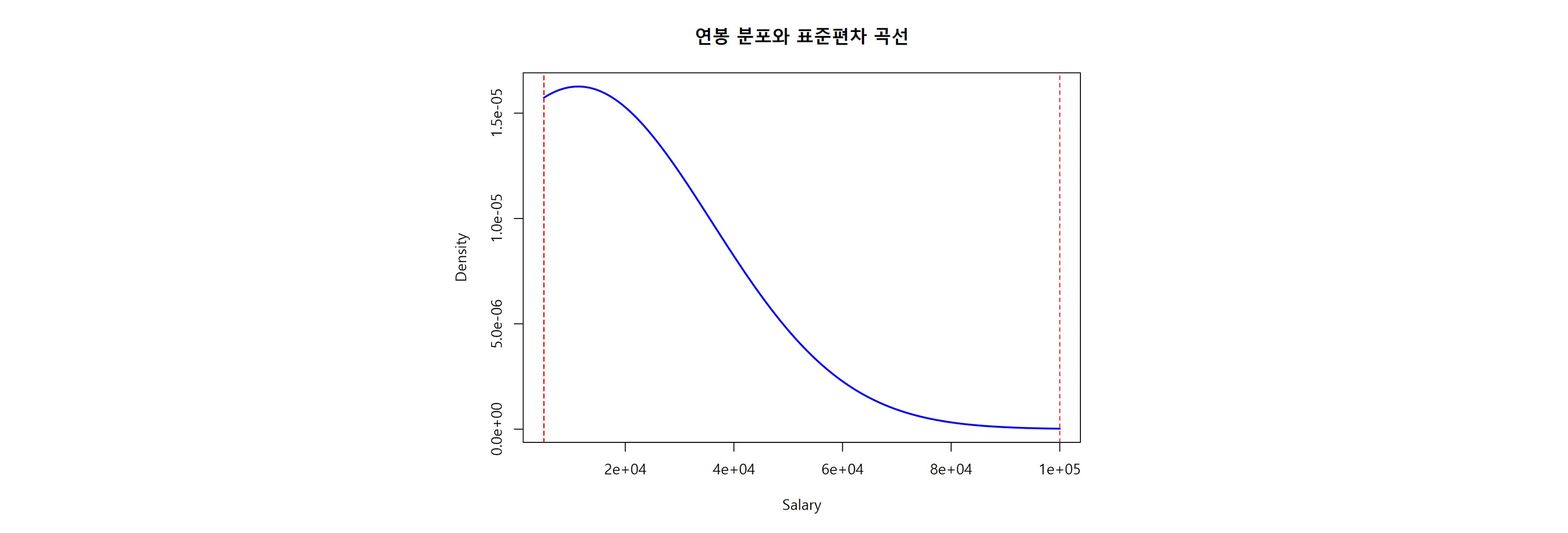
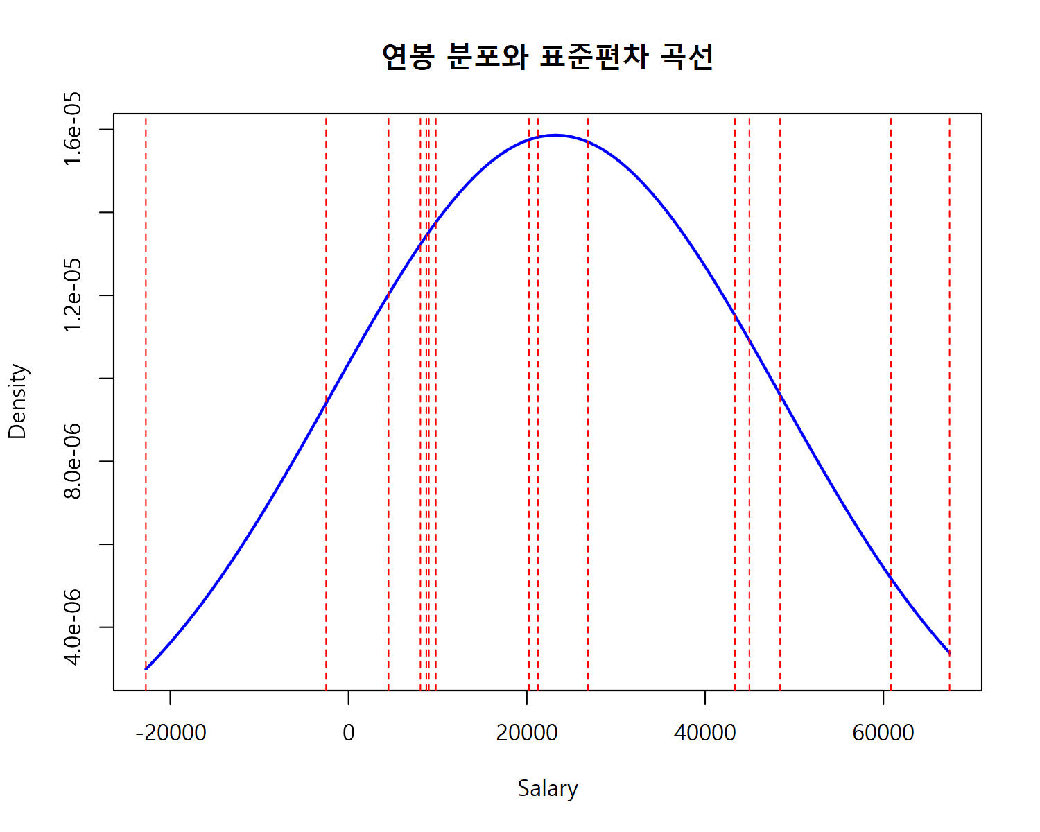
Population and sample · 5/5
## 07\. What is descriptive statistics?
### Supporting text from the original screen
07 / 77
Descriptive statistics · 1/8
## 08\. Descriptive statistics
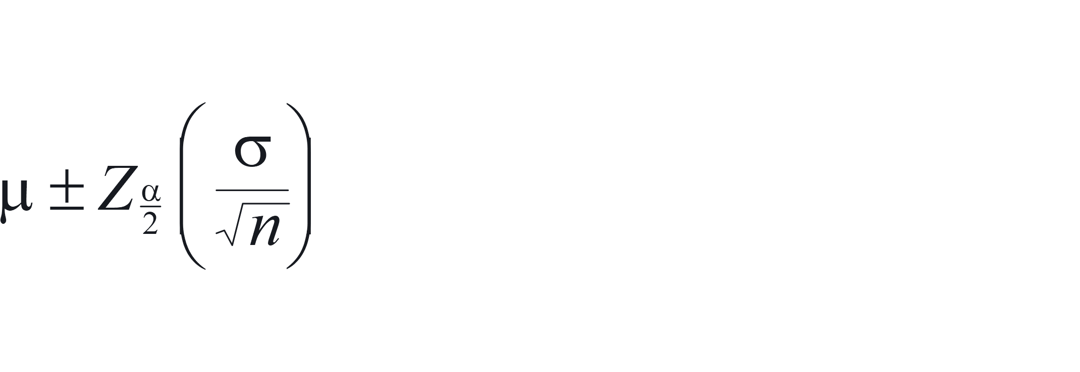
**Descriptive Statistics**
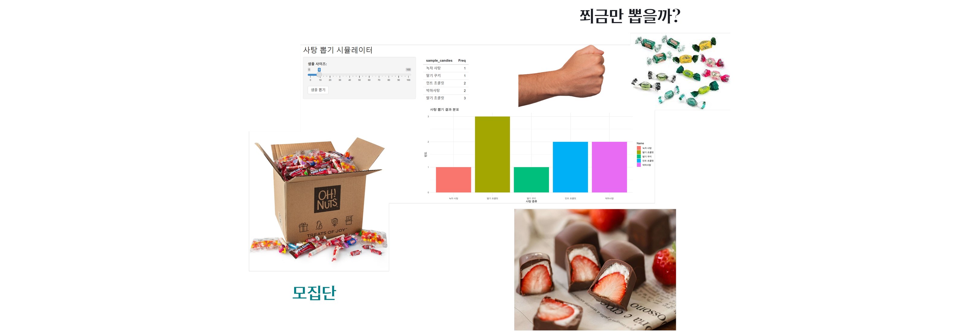
* A statistical method that identifies the characteristics of data through the organization, presentation, summarization, interpretation, etc. of data collected from measurements or experiments
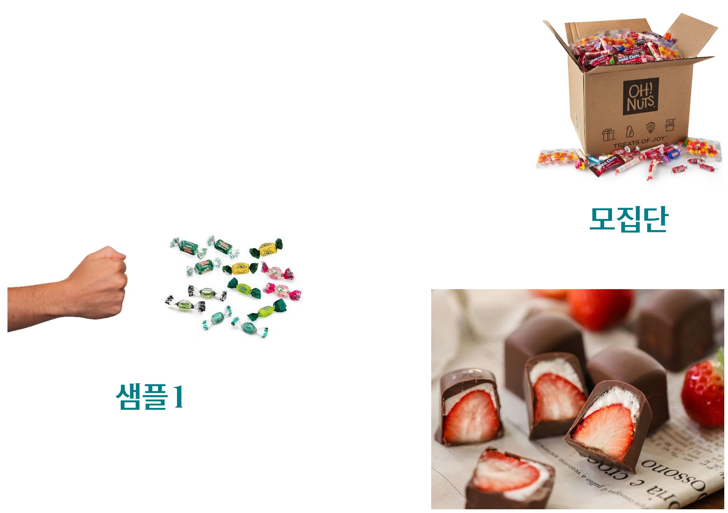
* A method of organizing the information contained in data through numerical summaries (sum, mean, variance, median, etc.) or graphical summaries of data obtained from the entire population or from a sample (sample: part of the population)
* Explaining the characteristics of data based on their basic statistical information

In the top row, an arrow goes from “Population” to “Parameter”; in the bottom row, from “Sample” to “Sample statistics”. Both arrows are labeled “Descriptive statistics”.
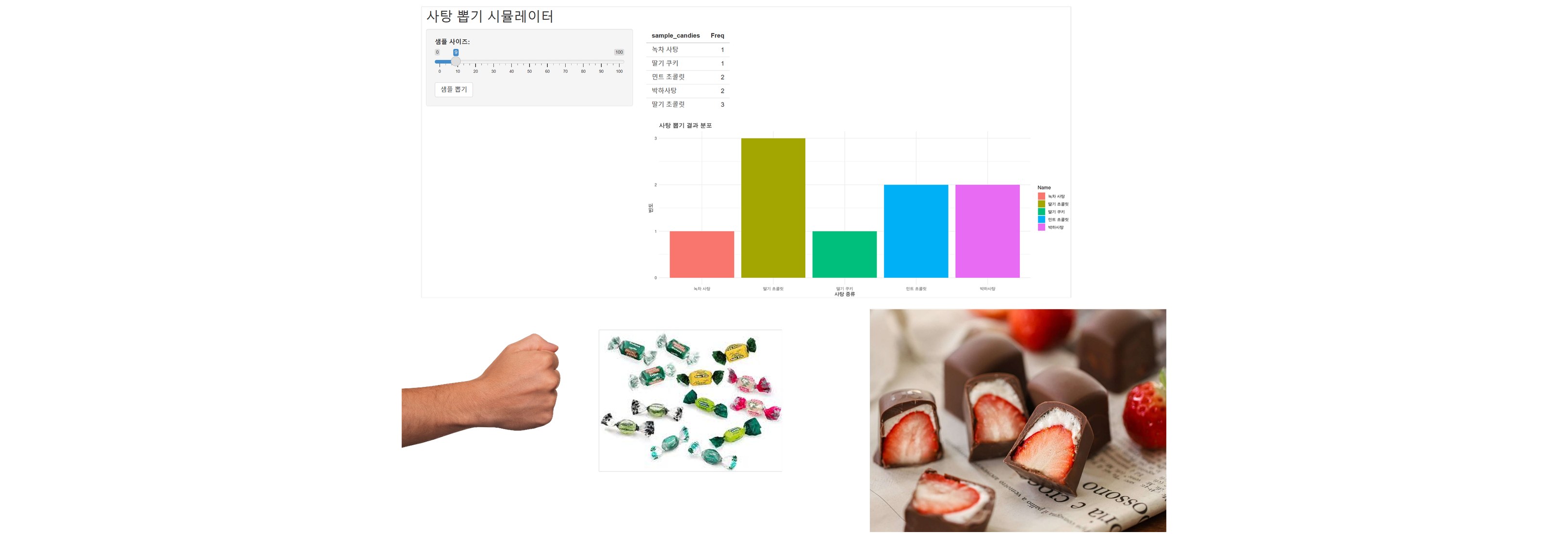
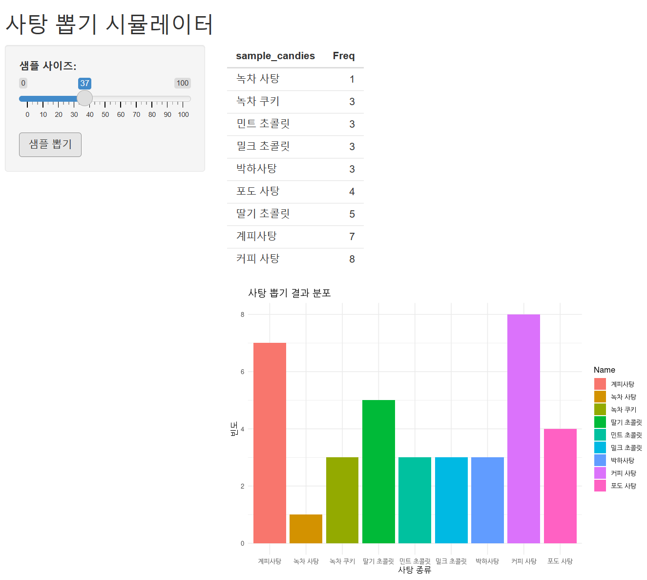
### Supporting text from the original screen
08 / 77
Descriptive statistics · 2/8
## 09\. Descriptive statistics
**Descriptive Statistics**
* Describing the data as they are
* Not a 3-line summary… but (mostly) a one-line summary
### Supporting text from the original screen
09 / 77
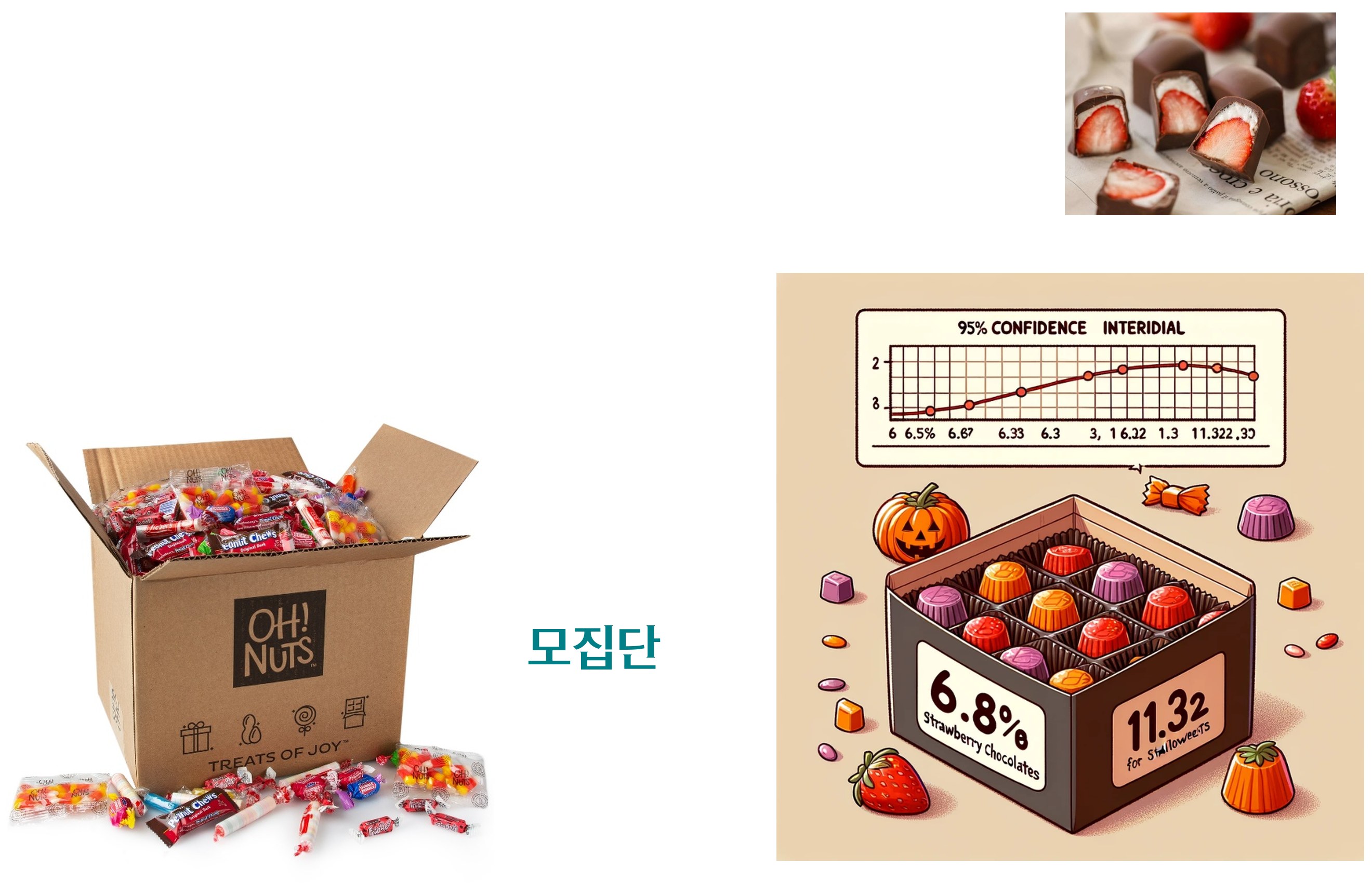
Descriptive statistics · 3/8
## 10\. Population and sample – candy-drawing simulator
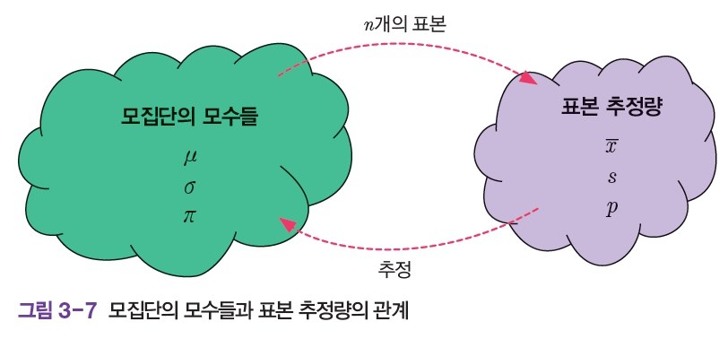
> What I drew with my fist came out as nothing but strawberry chocolates – but the box had an even mix?
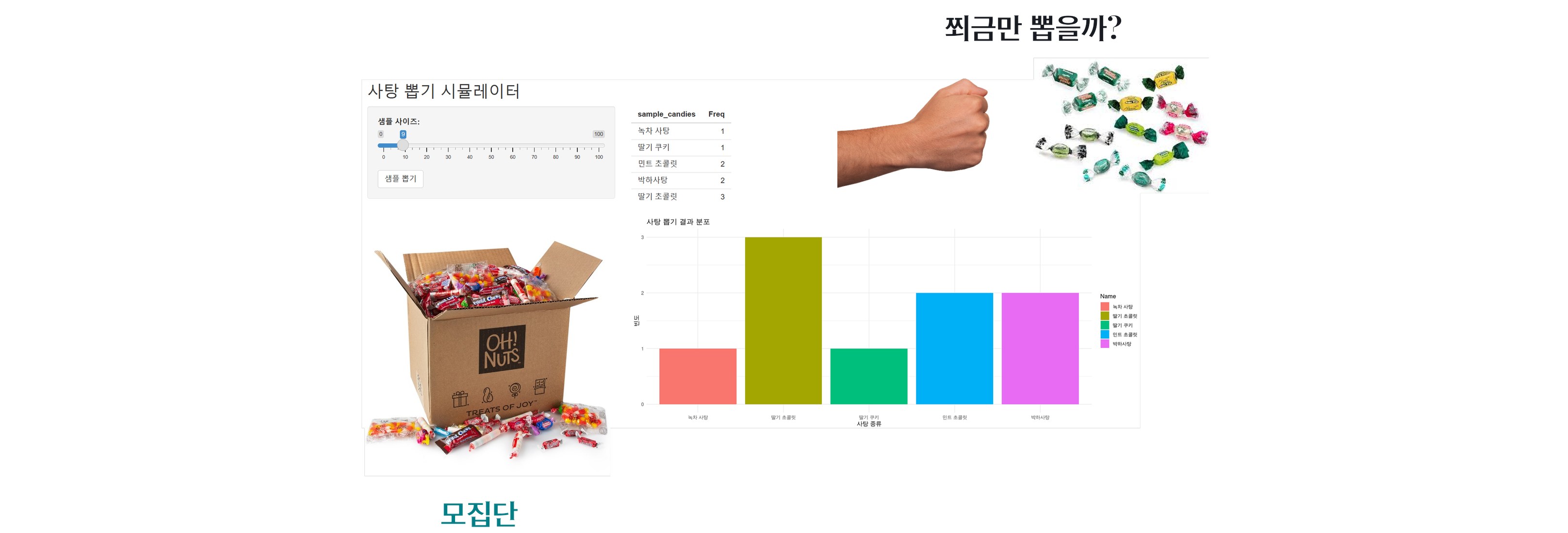
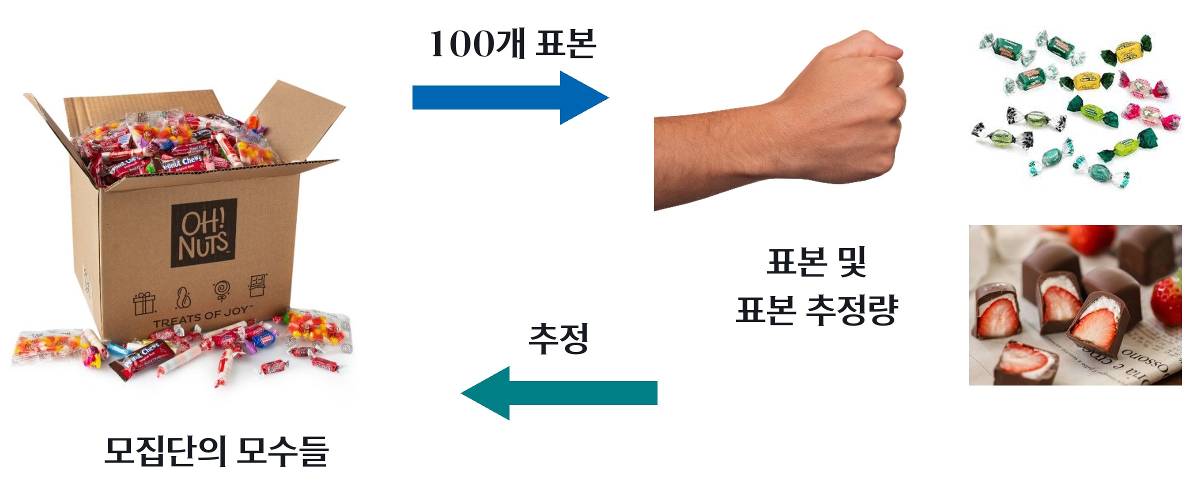
Overlaid on the candy-drawing simulator screen are ‘Shall we grab just a tiny handful?’ with a fist and a few candies on the right, and a photo of the candy box (population) at the bottom left. Candy-drawing simulator screen: at the top left, a slider for the number to draw and a table of counts for each kind of candy drawn; below, a bar chart by kind
### Supporting text from the original screen
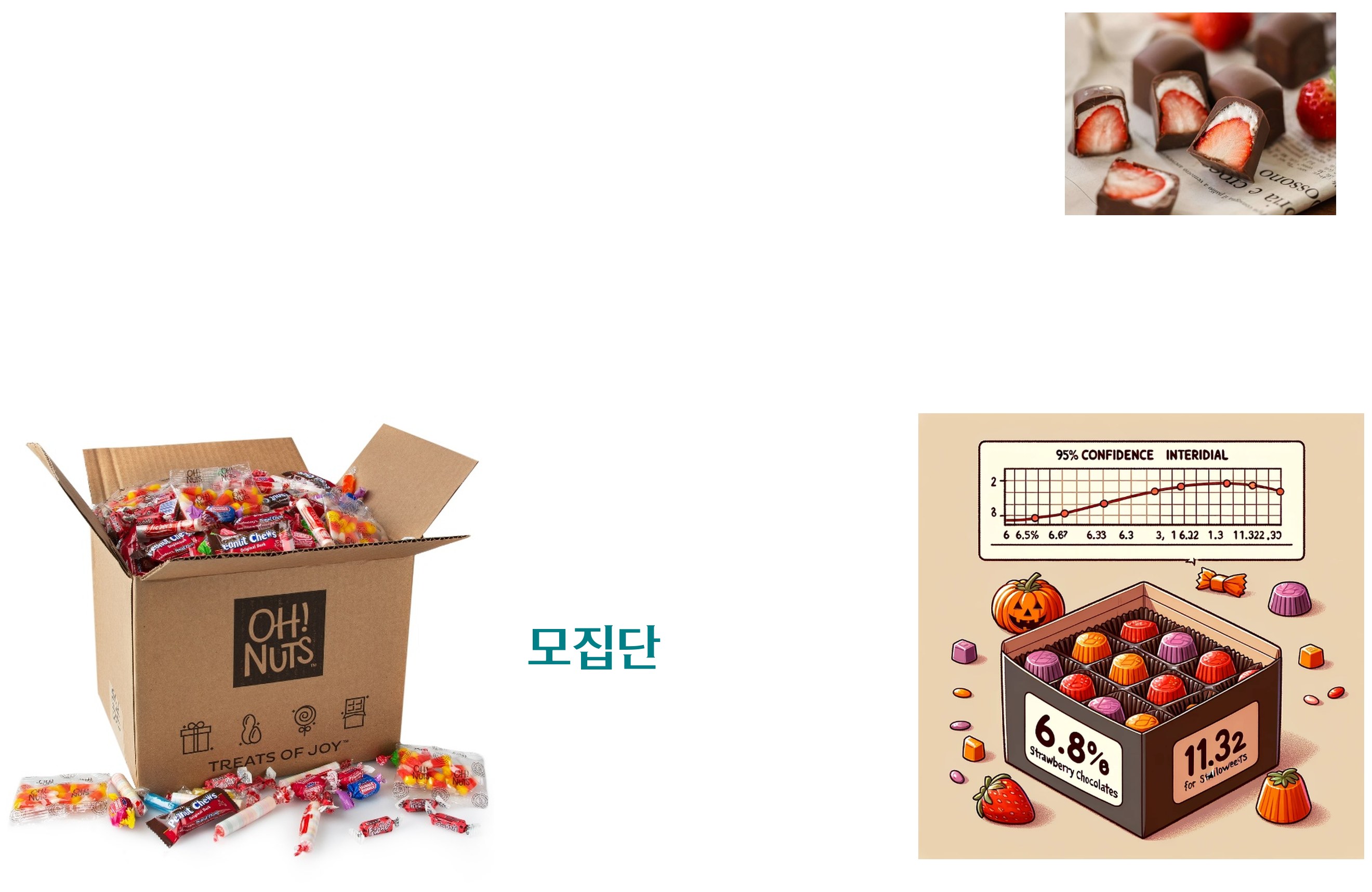
10 / 77
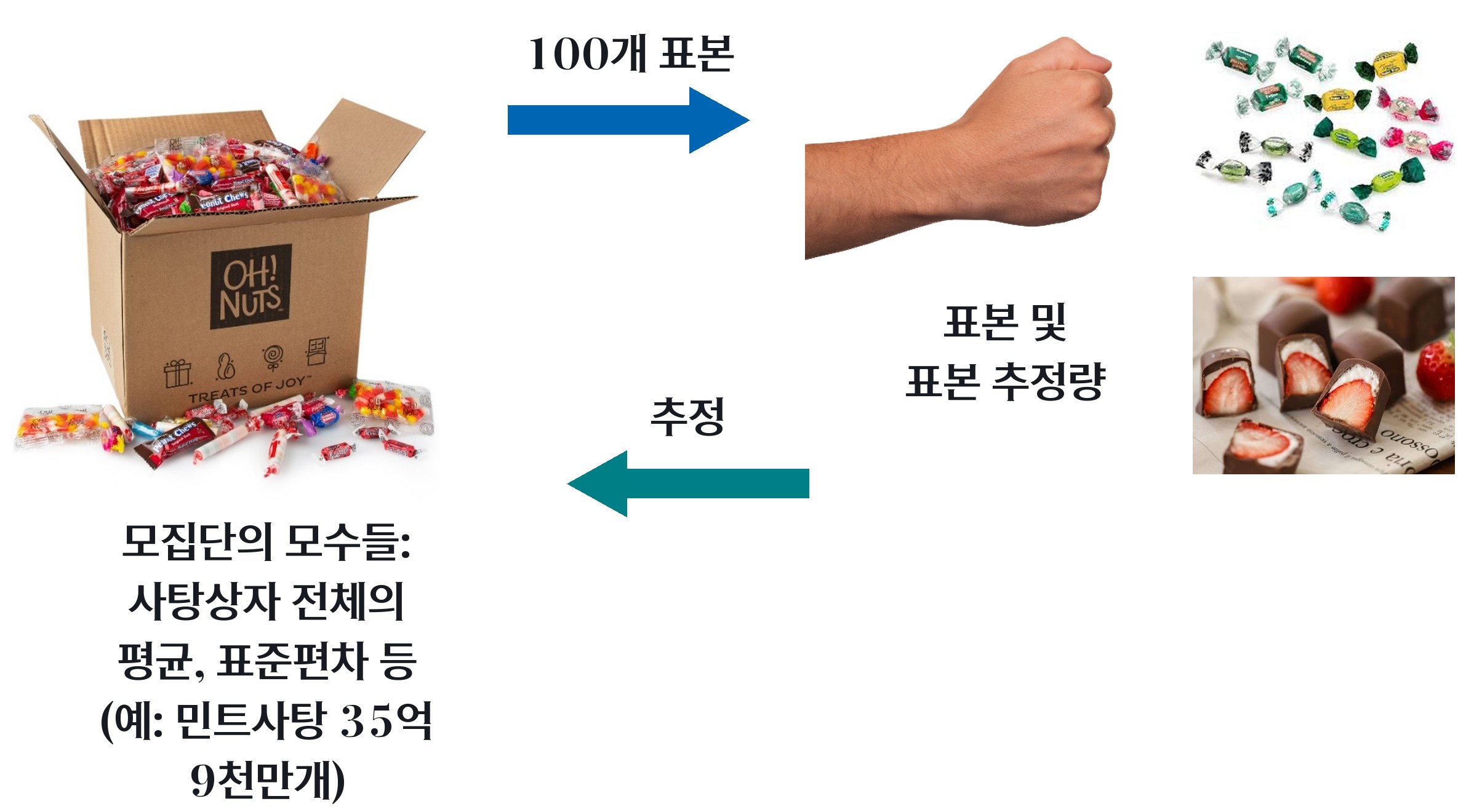
Descriptive statistics · 4/8
## 11\. Descriptive statistics
**Descriptive Statistics**
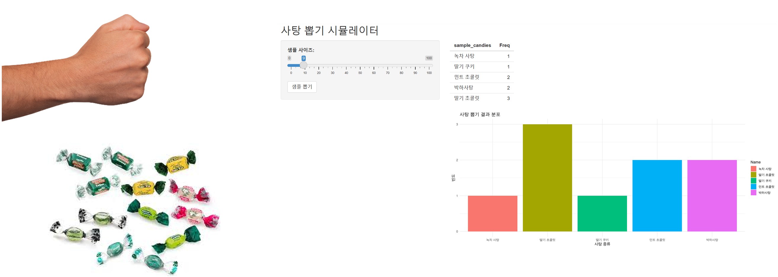
* Counting how many candies of each kind there are within the bunch of drawn candies,
* Calculating the mean count, median, mode, standard deviation, etc. for each kind of candy,
* Graphing the distribution of each kind of candy, and so on,
* The work of concretely identifying the characteristics within the bunch of drawn candies (the sample)
### Supporting text from the original screen
11 / 77
Descriptive statistics · 5/8
## 12\. Types and interpretation of descriptive statistics – what to use for a ‘one-line summary’
Descriptive statistics (expressing the characteristics of data in numbers)
**Central Tendency**
* Mode
* Median
* Mean
**Dispersion**
* Range
* Variance
* Standard deviation
**Distribution**
* Kurtosis
* Skewness
### Supporting text from the original screen
12 / 77
Descriptive statistics · 6/8
## 13\. Types and interpretation of descriptive statistics
**Descriptive statistics – Central Tendency**
Statistics that address which value represents the collected data, or around which value the data are concentrated
| Mode | The value with the highest frequency among all the data |
| --- | --- |
| Median | The value located exactly in the middle when all the data are arranged in rank order from the lowest value to the highest |
| Mean | The value obtained by adding up all the data and then dividing the total by the number of data points |
### Supporting text from the original screen
13 / 77
Descriptive statistics · 7/8
## 14\. Types and interpretation of descriptive statistics
**Mean**
Table 2-2 Monthly sales and number of purchases for shopping malls A and B
| Shopping mall | A | B |
| --- | --- | --- |
| Monthly sales | 3,000,000 won | 3,000,000 won |
| Monthly purchases | 100 purchases | 100 purchases |
| Average amount per purchase | 30,000 won | 30,000 won |
Table 2-3 Monthly sales and number of purchases for shopping malls A and B after free shipping for orders of 35,000 won or more
| Shopping mall | A | B |
| --- | --- | --- |
| Monthly sales | 3,300,000 won | 6,000,000 won |
| Monthly purchases | 110 purchases | 120 purchases |
| Average amount per purchase | 30,000 won | 50,000 won |
### Supporting text from the original screen
14 / 77
Descriptive statistics · 8/8
## 15\. Why R?
R (Quantitative Finance)
* Software specialized in performing statistical analysis, like SPSS
* With SPSS you pay a very high price every month, but R is open source (free)
* It can run almost all of the most complex statistics performed in SPSS
* The only drawback: R requires a little coding knowledge
* But if you use GPT, even that drawback drops in difficulty to the point where you hardly need to learn R coding at all
### Supporting text from the original screen
15 / 77
R and descriptive statistics · 1/22
## 16\. Installing R & R-Studio
[https://posit.co/download/rstudio-desktop/](https://posit.co/download/rstudio-desktop/)
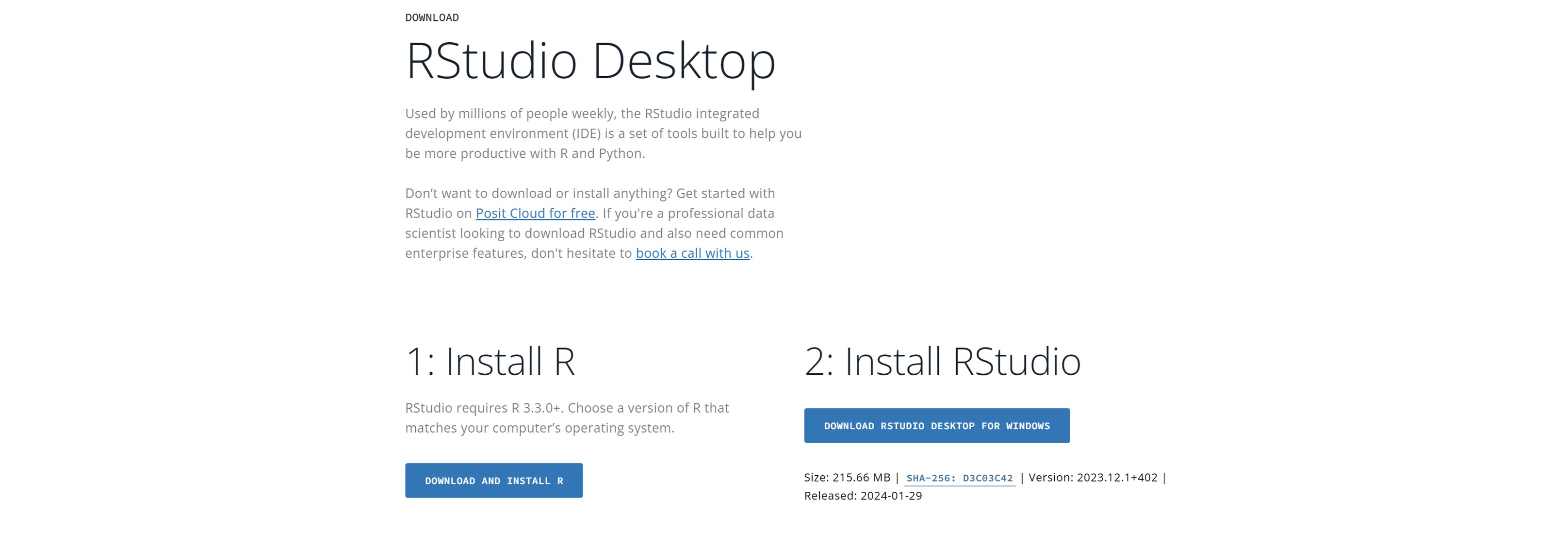
RStudio Desktop download page: the two steps ‘1: Install R’ and ‘2: Install RStudio’ with download buttons
### Supporting text from the original screen
16 / 77
R and descriptive statistics · 2/22
## 17\. Installing R & R-Studio
[https://cran.rstudio.com/](https://cran.rstudio.com/)
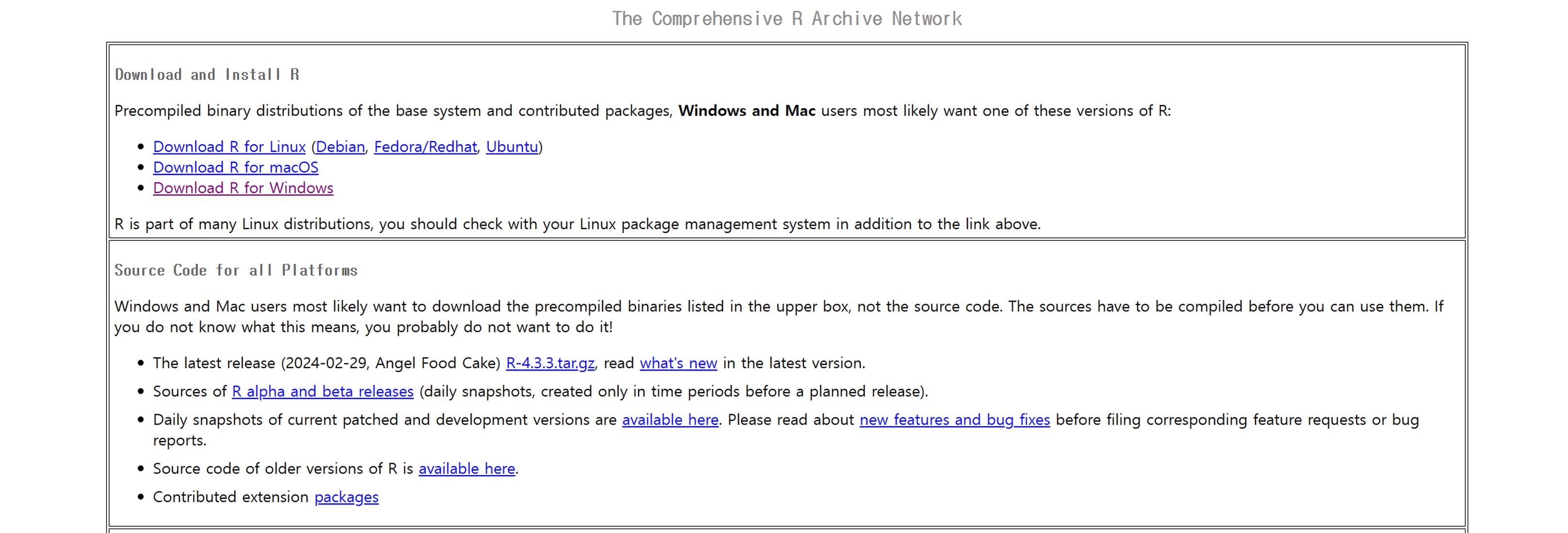
CRAN (The Comprehensive R Archive Network) front page: links to download R for Linux · macOS · Windows
### Supporting text from the original screen
17 / 77
R and descriptive statistics · 3/22
## 18\. Installing R & R-Studio
[https://cran.rstudio.com/](https://cran.rstudio.com/)
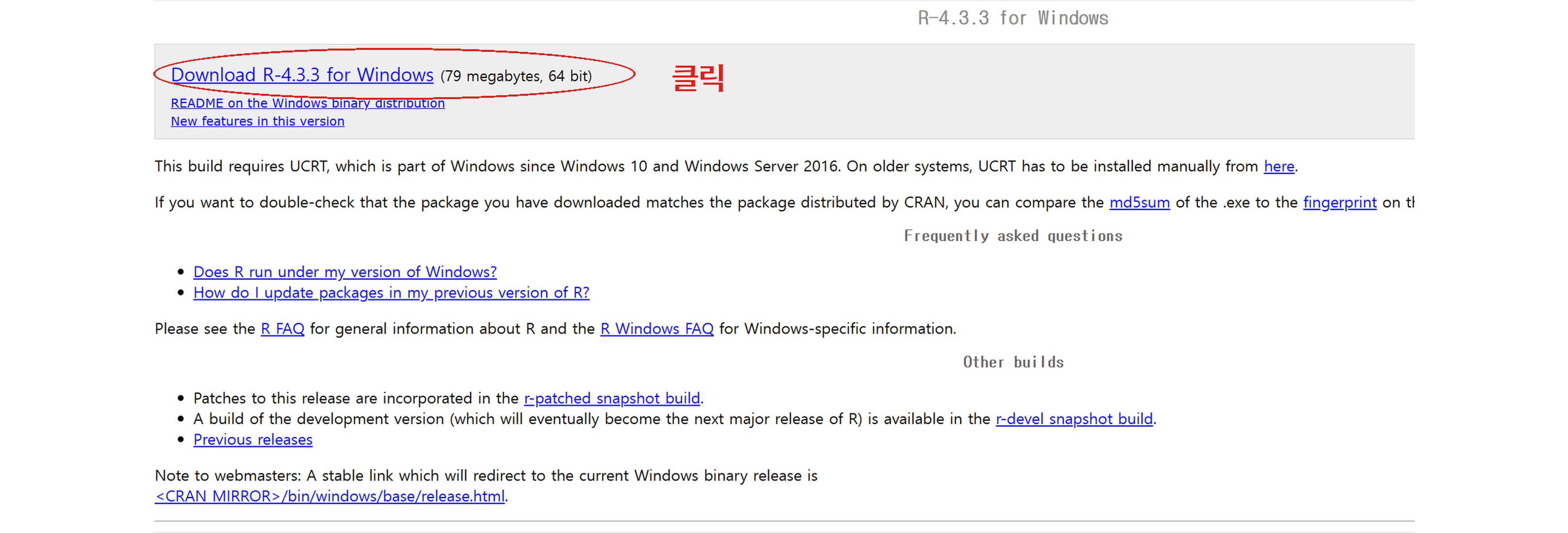
The ‘R-4.3.3 for Windows’ page. The ‘Download R-4.3.3 for Windows’ link at the very top is marked with a red circle and ‘Click’
### Supporting text from the original screen
18 / 77
R and descriptive statistics · 4/22
## 19\. Installing R & R-Studio
[https://cran.rstudio.com/](https://cran.rstudio.com/)
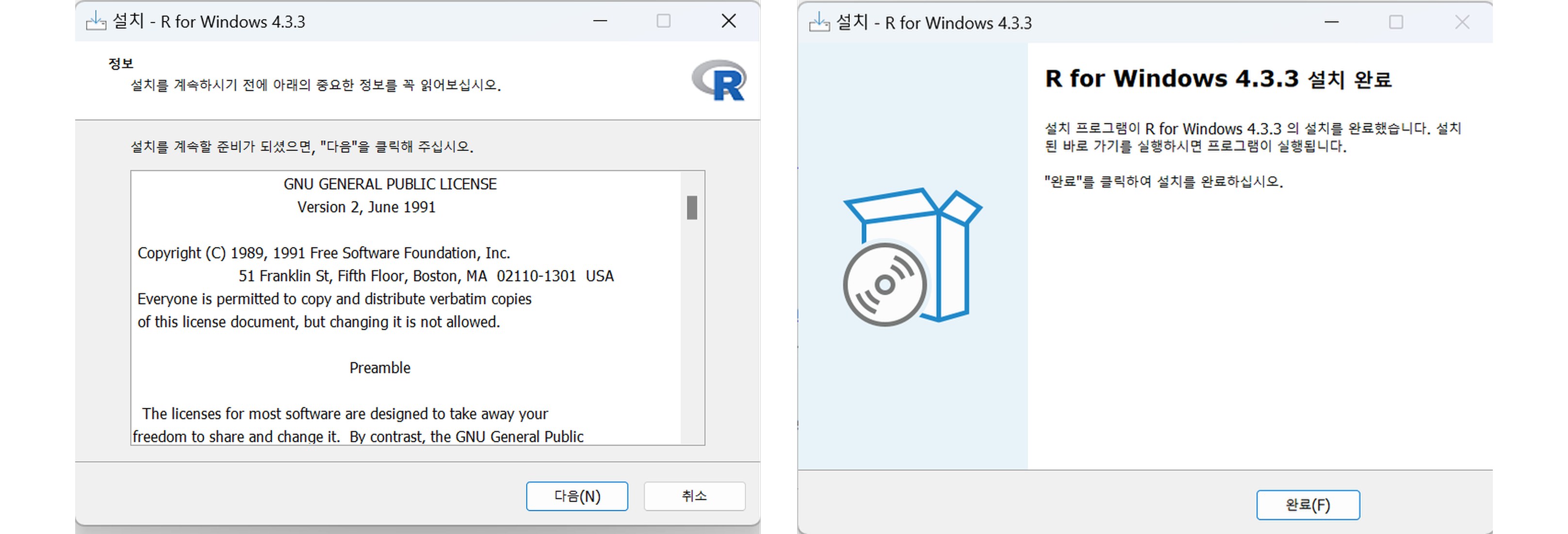
Two R for Windows 4.3.3 setup screens: on the left, the step for accepting the GNU General Public License; on the right, the setup-complete screen
### Supporting text from the original screen
19 / 77
R and descriptive statistics · 5/22
## 20\. Installing R & R-Studio
[https://posit.co/download/rstudio-desktop/](https://posit.co/download/rstudio-desktop/)
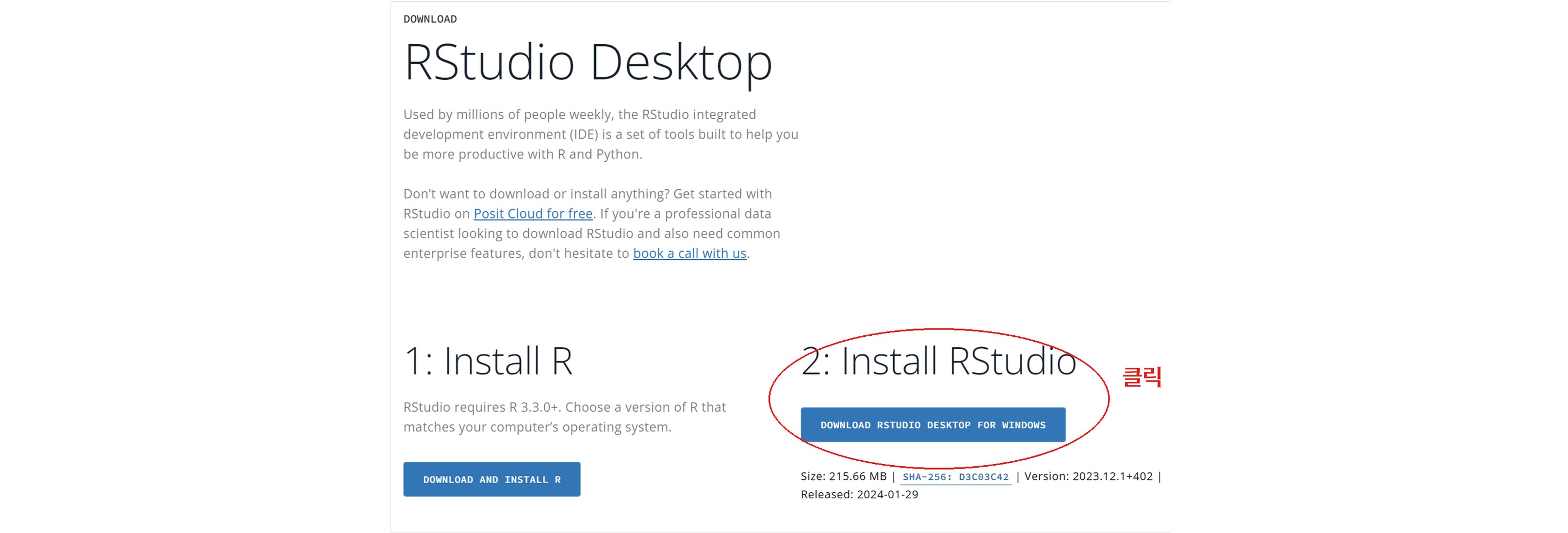
RStudio Desktop download page. The ‘2: Install RStudio’ button is marked with a red circle and ‘Click’
### Supporting text from the original screen
20 / 77
R and descriptive statistics · 6/22
## 21\. Installing R & R-Studio
[https://posit.co/download/rstudio-desktop/](https://posit.co/download/rstudio-desktop/)
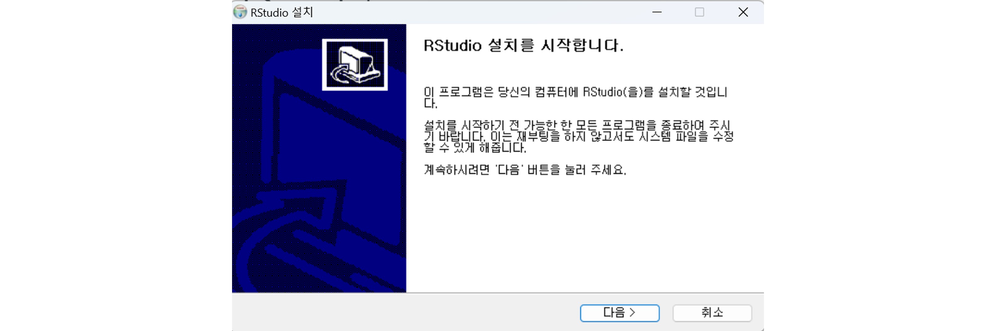
The ‘RStudio Setup’ start screen: the message ‘Starting RStudio Setup’ and the Next button
### Supporting text from the original screen
21 / 77
R and descriptive statistics · 7/22
## 22\. Running R-Studio
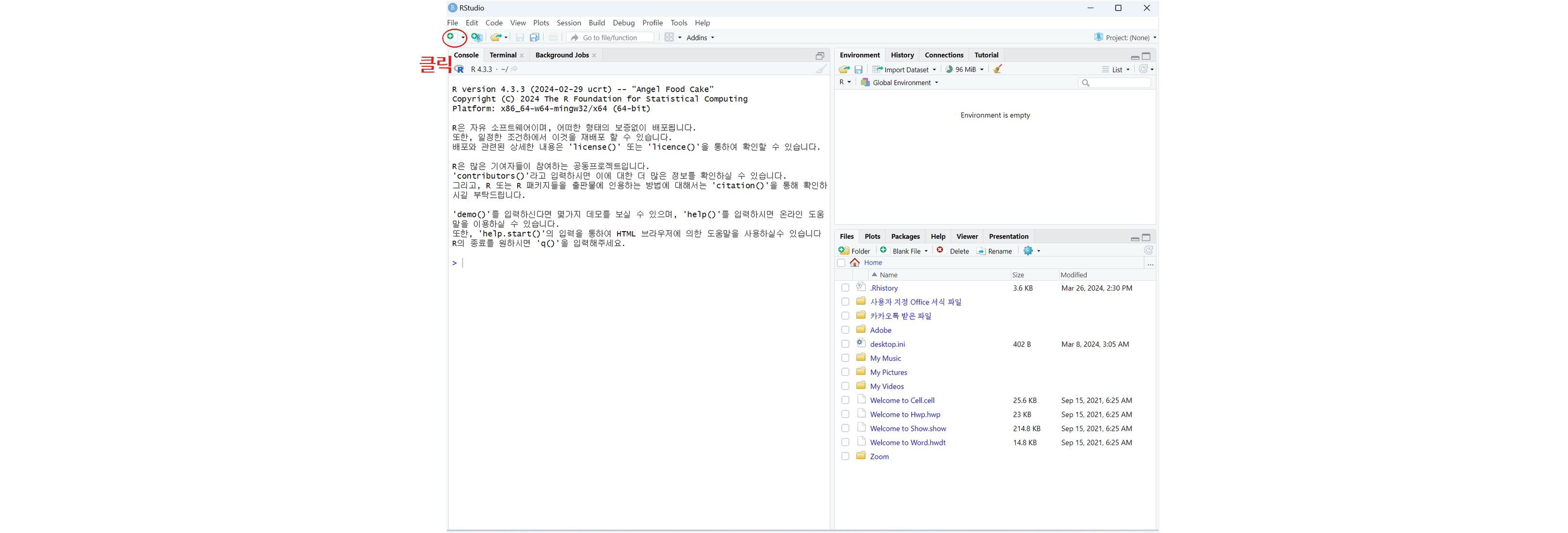
RStudio on first launch. The New File button at the top left is marked with a red circle and ‘Click’
### Supporting text from the original screen
22 / 77
R and descriptive statistics · 8/22
## 23\. Running R-Studio
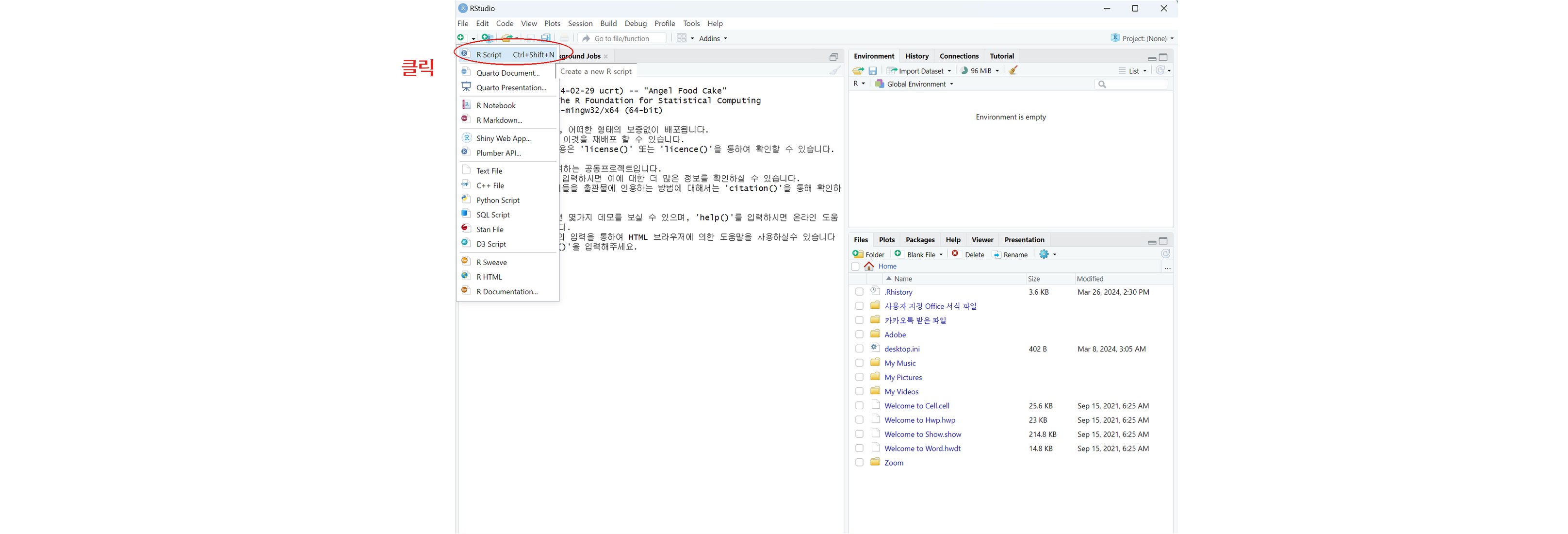
RStudio with the New File menu open. The ‘R Script’ item at the very top is marked with a red circle and ‘Click’
### Supporting text from the original screen
23 / 77
R and descriptive statistics · 9/22
## 24\. Running R-Studio
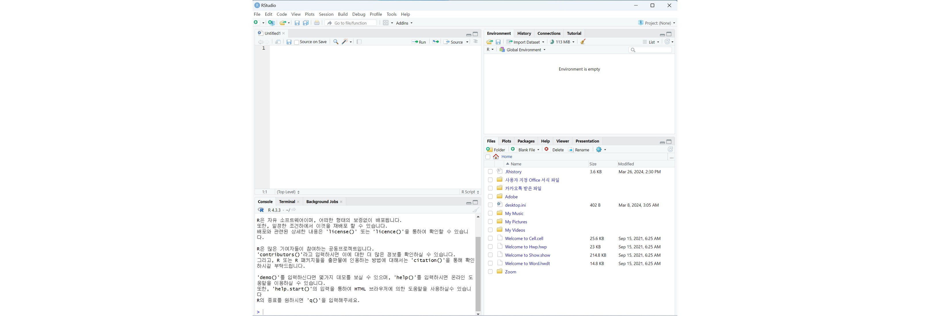
RStudio with an empty R script pane open
### Supporting text from the original screen
24 / 77
R and descriptive statistics · 10/22
## 25\. Running R-Studio: Ctrl+C / Ctrl+V the following code as is
```r
student_data <- data.frame(
name = c("학생1", "학생2", "학생3", "학생4", "학생5", "학생6", "학생7", "학생8",
"학생9", "학생10", "학생11", "학생12", "학생13", "학생14", "학생15"),
phone_usage = c(7.2, 5.8, 6.5, 8.1, 4.3, 6.7, 7.9, 5.2, 6.0, 7.5, 5.6, 6.3, 8.5, 5.0, 24.0),
age = c(20, 21, 19, 22, 20, 21, 20, 19, 22, 21, 20, 23, 19, 21, 20),
major = c("경영학", "컴퓨터공학", "영문학", "물리학", "화학공학", "통계학", "경제학",
"정치외교학", "생명과학", "전자공학", "국문학", "수학", "건축공학", "심리학", "사회학"))
```
### Supporting text from the original screen
25 / 77
R and descriptive statistics · 11/22
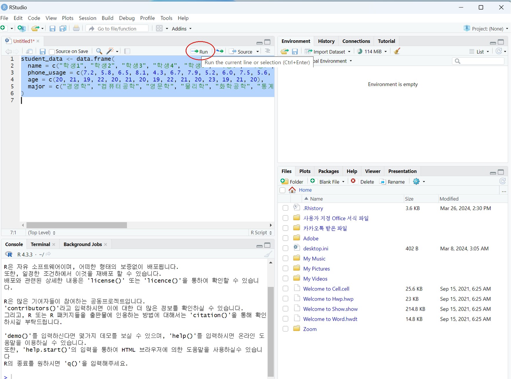
## 26\. Running R-Studio: Ctrl+C / Ctrl+V the following code as is
**Select all and click Run**
Or Ctrl+Enter
### Supporting text from the original screen
26 / 77
R and descriptive statistics · 12/22
## 27\. Example data for descriptive statistics
| name | phone\_usage | age | major |
| --- | --- | --- | --- |
| Student 1 | 7.2 | 20 | Business administration |
| Student 2 | 5.8 | 21 | Computer engineering |
| Student 3 | 6.5 | 19 | English literature |
| Student 4 | 8.1 | 22 | Physics |
| Student 5 | 4.3 | 20 | Chemical engineering |
| Student 6 | 6.7 | 21 | Statistics |
| Student 7 | 7.9 | 20 | Economics |
| Student 8 | 5.2 | 19 | Political science and diplomacy |
| name | phone\_usage | age | major |
| --- | --- | --- | --- |
| Student 9 | 6.0 | 22 | Life sciences |
| Student 10 | 7.5 | 21 | Electronic engineering |
| Student 11 | 5.6 | 20 | Korean literature |
| Student 12 | 6.3 | 23 | Mathematics |
| Student 13 | 8.5 | 19 | Architectural engineering |
| Student 14 | 5.0 | 21 | Psychology |
| Student 15 | 24.0 | 20 | Sociology |
### Supporting text from the original screen
27 / 77
R and descriptive statistics · 13/22
## 28\. Types and interpretation of descriptive statistics - mode
**Descriptive statistics – Central Tendency**
Statistics that address which value represents the collected data, or around which value the data are concentrated
| Mode | The value with the highest frequency among all the data |
| --- | --- |
| Median | The value located exactly in the middle when all the data are arranged in rank order from the lowest value to the highest |
| Mean | The value obtained by adding up all the data and then dividing the total by the number of data points |
### Supporting text from the original screen
28 / 77
R and descriptive statistics · 14/22
## 29\. AI & R Exercise - Mode
**Prompts:**
* “Find the mode of phone\_usage in this dataset”
* “To find the mode of phone\_usage in this dataset, count each value within that variable”
**Check with R code:**
```r
freq <- table(student_data$phone_usage)
maxfreq <- max(freq)
which(freq == maxfreq)
table(student_data$phone_usage)
```
**Check it with your own eyes**
**R output**
```text
> which(freq == maxfreq)
4.3 5 5.2 5.6 5.8 6 6.3 6.5 6.7 7.2 7.5 7.9 8.1
1 2 3 4 5 6 7 8 9 10 11 12 13
8.5 24
14 15
> table(student_data$phone_usage)
4.3 5 5.2 5.6 5.8 6 6.3 6.5 6.7 7.2 7.5 7.9 8.1
1 1 1 1 1 1 1 1 1 1 1 1 1
8.5 24
1 1
```
### Supporting text from the original screen
29 / 77
R and descriptive statistics · 15/22
## 30\. Example data for descriptive statistics – the answer for the mode
| name | phone\_usage | age | major |
| --- | --- | --- | --- |
| Student 1 | 7.2 | 20 | Business administration |
| Student 2 | 5.8 | 21 | Computer engineering |
| Student 3 | 6.5 | 19 | English literature |
| Student 4 | 8.1 | 22 | Physics |
| Student 5 | 4.3 | 20 | Chemical engineering |
| Student 6 | 6.7 | 21 | Statistics |
| Student 7 | 7.9 | 20 | Economics |
| Student 8 | 5.2 | 19 | Political science and diplomacy |
| name | phone\_usage | age | major |
| --- | --- | --- | --- |
| Student 9 | 6.0 | 22 | Life sciences |
| Student 10 | 7.5 | 21 | Electronic engineering |
| Student 11 | 5.6 | 20 | Korean literature |
| Student 12 | 6.3 | 23 | Mathematics |
| Student 13 | 8.5 | 19 | Architectural engineering |
| Student 14 | 5.0 | 21 | Psychology |
| Student 15 | 24.0 | 20 | Sociology |
Every value has a count of just 1
So there is no mode
### Supporting text from the original screen
30 / 77
R and descriptive statistics · 16/22
## 31\. Types and interpretation of descriptive statistics - median
**Descriptive statistics – Central Tendency**
Statistics that address which value represents the collected data, or around which value the data are concentrated
| Mode | The value with the highest frequency among all the data |
| --- | --- |
| Median | The value located exactly in the middle when all the data are arranged in rank order from the lowest value to the highest |
| Mean | The value obtained by adding up all the data and then dividing the total by the number of data points |
### Supporting text from the original screen
31 / 77
R and descriptive statistics · 17/22
## 32\. AI & R Exercise - Median
**Prompts:**
* “Find the median of phone\_usage in this dataset”
* “To find the median of phone\_usage in this dataset, arrange each value within that variable in order from smallest to largest”
**Check with R code:**
```r
median(student_data$phone_usage)
```
**Check it with your own eyes**
**R output**
```text
> median(student_data$phone_usage)
[1] 6.5
```
### Supporting text from the original screen
32 / 77
R and descriptive statistics · 18/22
## 33\. Example data for descriptive statistics – the answer for the median
| name | phone\_usage | age | major |
| --- | --- | --- | --- |
| Student 5 | 4.3 | 20 | Chemical engineering |
| Student 14 | 5.0 | 21 | Psychology |
| Student 8 | 5.2 | 19 | Political science and diplomacy |
| Student 11 | 5.6 | 20 | Korean literature |
| Student 2 | 5.8 | 21 | Computer engineering |
| Student 9 | 6.0 | 22 | Life sciences |
| Student 12 | 6.3 | 23 | Mathematics |
| Student 3 | 6.5 | 19 | English literature |
| name | phone\_usage | age | major |
| --- | --- | --- | --- |
| Student 6 | 6.7 | 21 | Statistics |
| Student 1 | 7.2 | 20 | Business administration |
| Student 10 | 7.5 | 21 | Electronic engineering |
| Student 7 | 7.9 | 20 | Economics |
| Student 4 | 8.1 | 22 | Physics |
| Student 13 | 8.5 | 19 | Architectural engineering |
| Student 15 | 24.0 | 20 | Sociology |
6.5 is exactly the 8th value whether you count from the top or the bottom
So the median is 6.5
### Supporting text from the original screen
33 / 77
R and descriptive statistics · 19/22
## 34\. Types and interpretation of descriptive statistics - mean
**Descriptive statistics – Central Tendency**
Statistics that address which value represents the collected data, or around which value the data are concentrated
| Mode | The value with the highest frequency among all the data |
| --- | --- |
| Median | The value located exactly in the middle when all the data are arranged in rank order from the lowest value to the highest |
| Mean | The value obtained by adding up all the data and then dividing the total by the number of data points |
### Supporting text from the original screen
34 / 77
R and descriptive statistics · 20/22
## 35\. AI & R Exercise - Mean
**Prompts:**
* “Find the mean value of phone\_usage in this dataset”
* “Show the calculation steps for finding the mean value of phone\_usage in this dataset, and find the mean value”
**Check with R code:**
```r
mean(student_data$phone_usage)
```
**Check by calculating it yourself on a calculator**
**R output**
```text
> mean(student_data$phone_usage)
[1] 7.64
```
### Supporting text from the original screen
35 / 77
R and descriptive statistics · 21/22
## 36\. Example data for descriptive statistics – the answer for the mean value
| name | phone\_usage | age | major |
| --- | --- | --- | --- |
| Student 5 | 4.3 | 20 | Chemical engineering |
| Student 14 | 5.0 | 21 | Psychology |
| Student 8 | 5.2 | 19 | Political science and diplomacy |
| Student 11 | 5.6 | 20 | Korean literature |
| Student 2 | 5.8 | 21 | Computer engineering |
| Student 9 | 6.0 | 22 | Life sciences |
| Student 12 | 6.3 | 23 | Mathematics |
| Student 3 | 6.5 | 19 | English literature |
| name | phone\_usage | age | major |
| --- | --- | --- | --- |
| Student 6 | 6.7 | 21 | Statistics |
| Student 1 | 7.2 | 20 | Business administration |
| Student 10 | 7.5 | 21 | Electronic engineering |
| Student 7 | 7.9 | 20 | Economics |
| Student 4 | 8.1 | 22 | Physics |
| Student 13 | 8.5 | 19 | Architectural engineering |
| Student 15 | 24.0 | 20 | Sociology |
Sum of all values: 114.6
The sum divided by 15: 7.64
### Supporting text from the original screen
36 / 77
R and descriptive statistics · 22/22
## 37\. The trap of the mean
### Supporting text from the original screen
37 / 77
The trap of the mean · 1/18
## 38\. Example data for descriptive statistics – the problem with the mean value: Outlier
| name | phone\_usage | age | major |
| --- | --- | --- | --- |
| Student 5 | 4.3 | 20 | Chemical engineering |
| Student 14 | 5.0 | 21 | Psychology |
| Student 8 | 5.2 | 19 | Political science and diplomacy |
| Student 11 | 5.6 | 20 | Korean literature |
| Student 2 | 5.8 | 21 | Computer engineering |
| Student 9 | 6.0 | 22 | Life sciences |
| Student 12 | 6.3 | 23 | Mathematics |
| Student 3 | 6.5 | 19 | English literature |
| name | phone\_usage | age | major |
| --- | --- | --- | --- |
| Student 6 | 6.7 | 21 | Statistics |
| Student 1 | 7.2 | 20 | Business administration |
| Student 10 | 7.5 | 21 | Electronic engineering |
| Student 7 | 7.9 | 20 | Economics |
| Student 4 | 8.1 | 22 | Physics |
| Student 13 | 8.5 | 19 | Architectural engineering |
| Student 15 | 24.0 | 20 | Sociology |
1 student uses a smartphone for 24 hours · What if we leave this student out and recalculate? 90.6 / 14 = 6.47
**The students' average smartphone time is 6.5 hours, not 7.6 hours.**
### Supporting text from the original screen
38 / 77
The trap of the mean · 2/18
## 39\. R-Studio example 2: Ctrl+C / Ctrl+V the following code as is
```r
student_data <- data.frame(
name = c("학생1", "학생2", "학생3", "학생4", "학생5", "학생6", "학생7", "학생8",
"학생9", "학생10", "학생11", "학생12", "학생13", "학생14", "학생15"),
phone_usage = c(7.2, 5.8, 6.5, 8.1, 4.3, 6.7, 7.9, 5.2, 6.0, 7.5, 5.6, 6.3, 8.5, 5.0, 24.0),
age = c(20, 21, 19, 22, 20, 21, 20, 19, 22, 21, 20, 23, 19, 21, 20),
major = c("경영학", "컴퓨터공학", "영문학", "물리학", "화학공학", "통계학", "경제학",
"정치외교학", "생명과학", "전자공학", "국문학", "수학", "건축공학", "심리학", "사회학"),
salary = c(rep(5000, 14), 100000)
)
```
### Supporting text from the original screen
39 / 77
The trap of the mean · 3/18
## 40\. R-Studio example 2: salary
| name | phone\_usage | age | major | salary |
| --- | --- | --- | --- | --- |
| Student 1 | 7.2 | 20 | Business administration | 5000 |
| Student 2 | 5.8 | 21 | Computer engineering | 5000 |
| Student 3 | 6.5 | 19 | English literature | 5000 |
| Student 4 | 8.1 | 22 | Physics | 5000 |
| Student 5 | 4.3 | 20 | Chemical engineering | 5000 |
| Student 6 | 6.7 | 21 | Statistics | 5000 |
| Student 7 | 7.9 | 20 | Economics | 5000 |
| Student 8 | 5.2 | 19 | Political science and diplomacy | 5000 |
| name | phone\_usage | age | major | salary |
| --- | --- | --- | --- | --- |
| Student 9 | 6.0 | 22 | Life sciences | 5000 |
| Student 10 | 7.5 | 21 | Electronic engineering | 5000 |
| Student 11 | 5.6 | 20 | Korean literature | 5000 |
| Student 12 | 6.3 | 23 | Mathematics | 5000 |
| Student 13 | 8.5 | 19 | Architectural engineering | 5000 |
| Student 14 | 5.0 | 21 | Psychology | 5000 |
| Student 15 | 24.0 | 20 | Sociology | 100000 |
### Supporting text from the original screen
40 / 77
The trap of the mean · 4/18
## 41\. AI & R Exercise - Mean
**Prompts:**
* “Find the mean value of salary in this dataset”
* “Show the calculation steps for finding the mean value of salary in this dataset, and find the mean value”
**Check with R code:**
```r
mean(student_data$salary)
```
**R output**
```text
> mean(student_data$salary)
[1] 11333.33
```
### Supporting text from the original screen
41 / 77
The trap of the mean · 5/18
## 42\. R-Studio example 2: the answer for the average salary
| name | phone\_usage | age | major | salary |
| --- | --- | --- | --- | --- |
| Student 1 | 7.2 | 20 | Business administration | 5000 |
| Student 2 | 5.8 | 21 | Computer engineering | 5000 |
| Student 3 | 6.5 | 19 | English literature | 5000 |
| Student 4 | 8.1 | 22 | Physics | 5000 |
| Student 5 | 4.3 | 20 | Chemical engineering | 5000 |
| Student 6 | 6.7 | 21 | Statistics | 5000 |
| Student 7 | 7.9 | 20 | Economics | 5000 |
| Student 8 | 5.2 | 19 | Political science and diplomacy | 5000 |
| name | phone\_usage | age | major | salary |
| --- | --- | --- | --- | --- |
| Student 9 | 6.0 | 22 | Life sciences | 5000 |
| Student 10 | 7.5 | 21 | Electronic engineering | 5000 |
| Student 11 | 5.6 | 20 | Korean literature | 5000 |
| Student 12 | 6.3 | 23 | Mathematics | 5000 |
| Student 13 | 8.5 | 19 | Architectural engineering | 5000 |
| Student 14 | 5.0 | 21 | Psychology | 5000 |
| Student 15 | 24.0 | 20 | Sociology | 100000 |
R-Studio code result: 11333.33
Annual salary per person: 113.33 million won
### Supporting text from the original screen
42 / 77
The trap of the mean · 6/18
## 43\. The trap of the mean
* Ah, the average salary came out to 113.33 million won, so Hallym University students' salaries average over 100 million won! = the trap of the mean
* Because of a single unusual person earning over 1 billion won, the average salary gets inflated
* That ‘unusual person’ throws the statistical results off, and in statistics such an ‘unusual person’ is called an Outlier
### Supporting text from the original screen
43 / 77
The trap of the mean · 7/18
## 44\. Median income in Korea
[https://www.index.go.kr/unify/idx-info.do?idxCd=8001](https://www.index.go.kr/unify/idx-info.do?idxCd=8001)
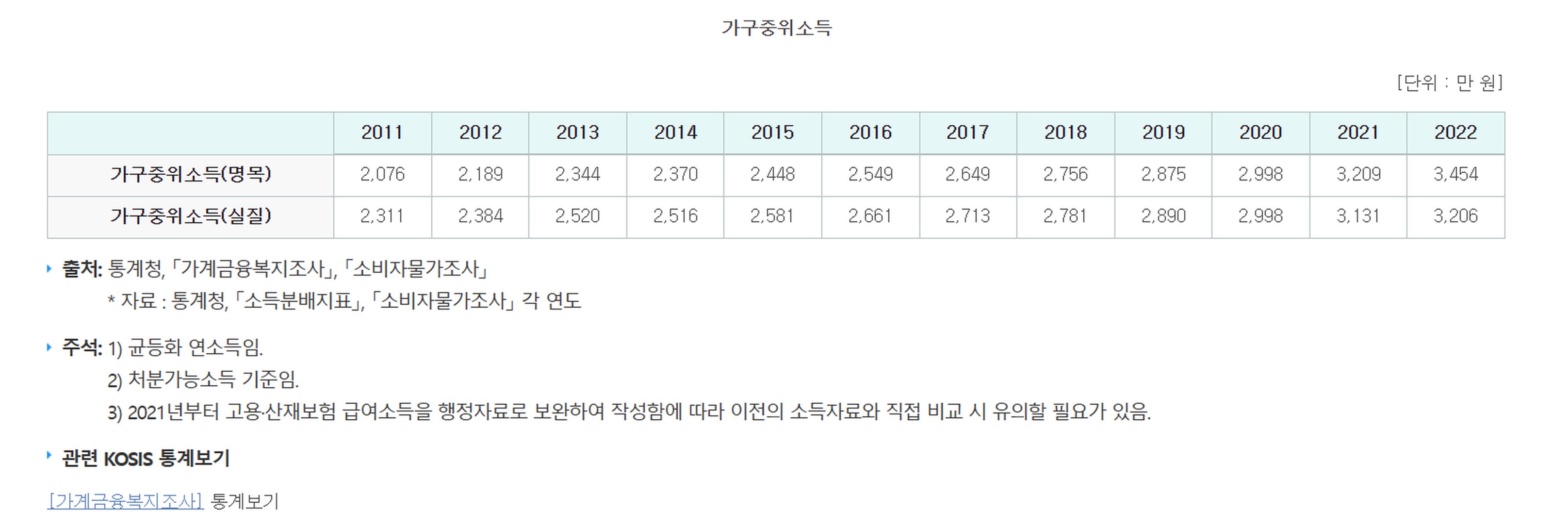
Screen of the ‘Household median income’ table in Korea's National Indicator System: household median income (nominal · real) for 2011–2022, with source · notes
### Supporting text from the original screen
44 / 77
The trap of the mean · 8/18
## 45\. Trends in Korea's standard median income (by household size)
[https://www.index.go.kr/unity/potal/main/EachDtlPageDetail.do?idx\_cd=2762](https://www.index.go.kr/unity/potal/main/EachDtlPageDetail.do?idx_cd=2762)
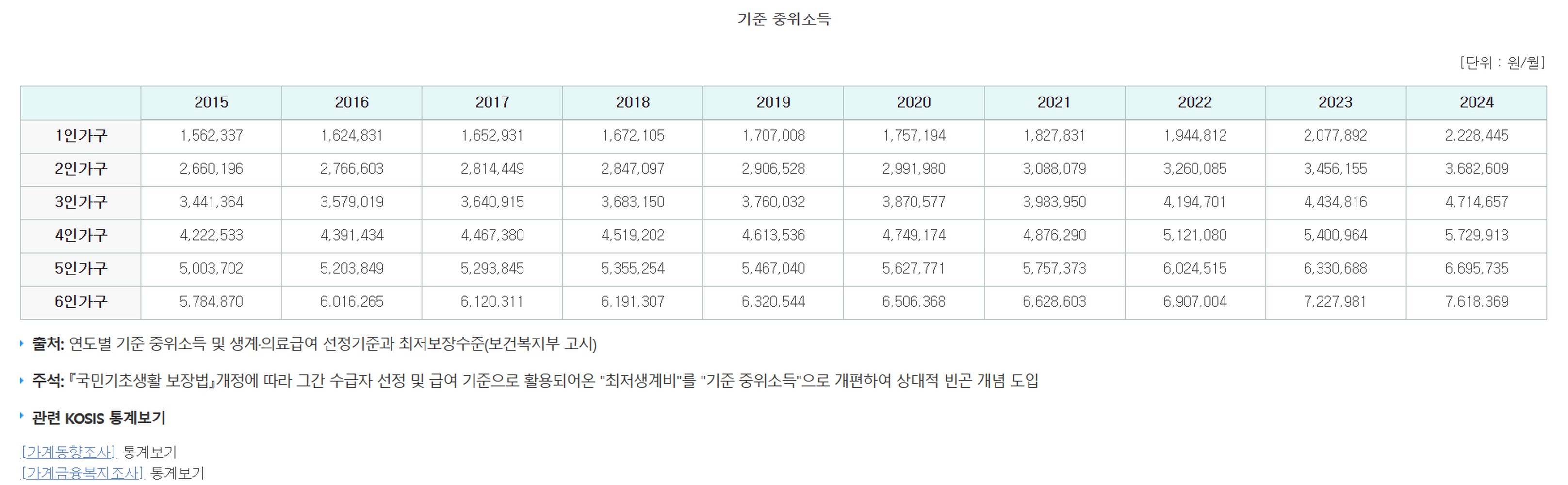
Screen of the ‘Standard median income’ table in Korea's National Indicator System: standard median income for households of 1 to 7 persons, 2015–2024, with source · notes
### Supporting text from the original screen
45 / 77
The trap of the mean · 9/18
## 46\. Types and interpretation of descriptive statistics
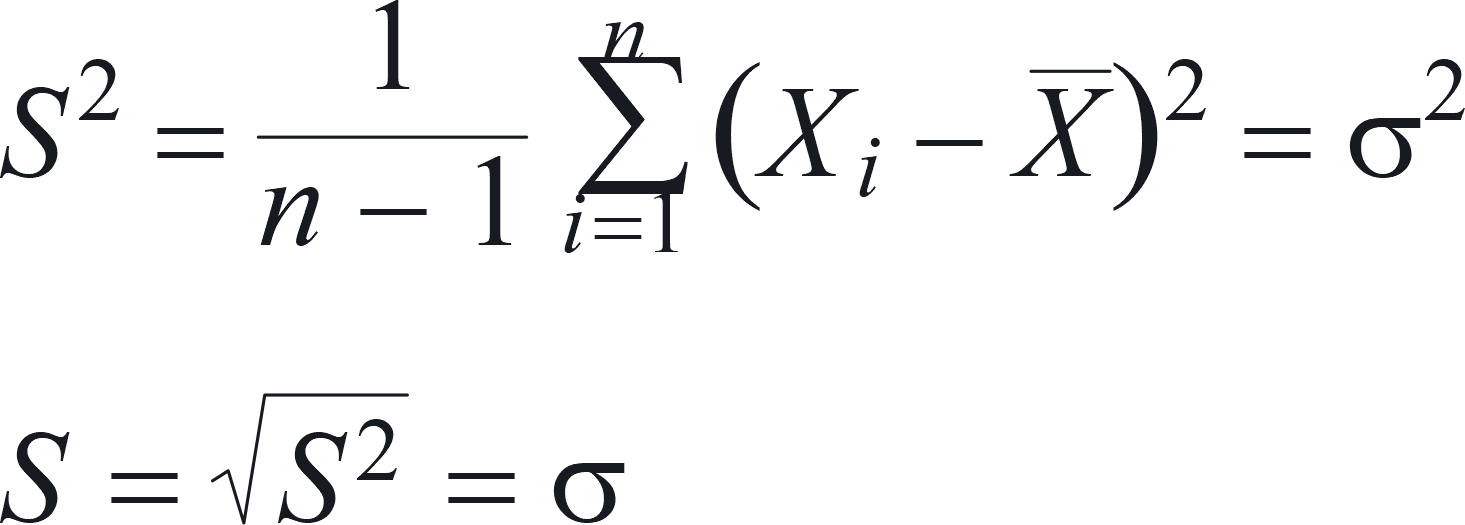
**Variance and standard deviation**
* Variance: uses the mean (X̄) as the reference for how spread out the data are
* Standard deviation: a measure used when calculating the proportion of data that fall within a certain distance of the mean
To put it more simply, a map that shows how the overall mean value is spread out when you line up the mean values horizontally from the low ones to the high ones
### Supporting text from the original screen
46 / 77
The trap of the mean · 10/18
## 47\. Types and interpretation of descriptive statistics
**The 68-95 rule**
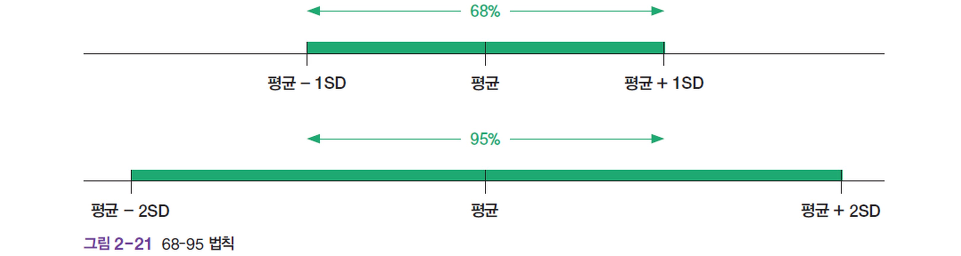
Figure 2-21 The 68-95 rule: two bars showing 68% from mean−1SD to mean+1SD and 95% from mean−2SD to mean+2SD
### Supporting text from the original screen
47 / 77
The trap of the mean · 11/18
## 48\. Types and interpretation of descriptive statistics
**Kurtosis**
Positive kurtosis:
turns out the folks who invested in Bitcoin are crowded tightly together
Negative kurtosis:
turns out lots of folks got burned on Bitcoin and sold at a loss, so there are fewer folks holding coins than last year
### Supporting text from the original screen
48 / 77
The trap of the mean · 12/18
## 49\. Types and interpretation of descriptive statistics
**Skewness**
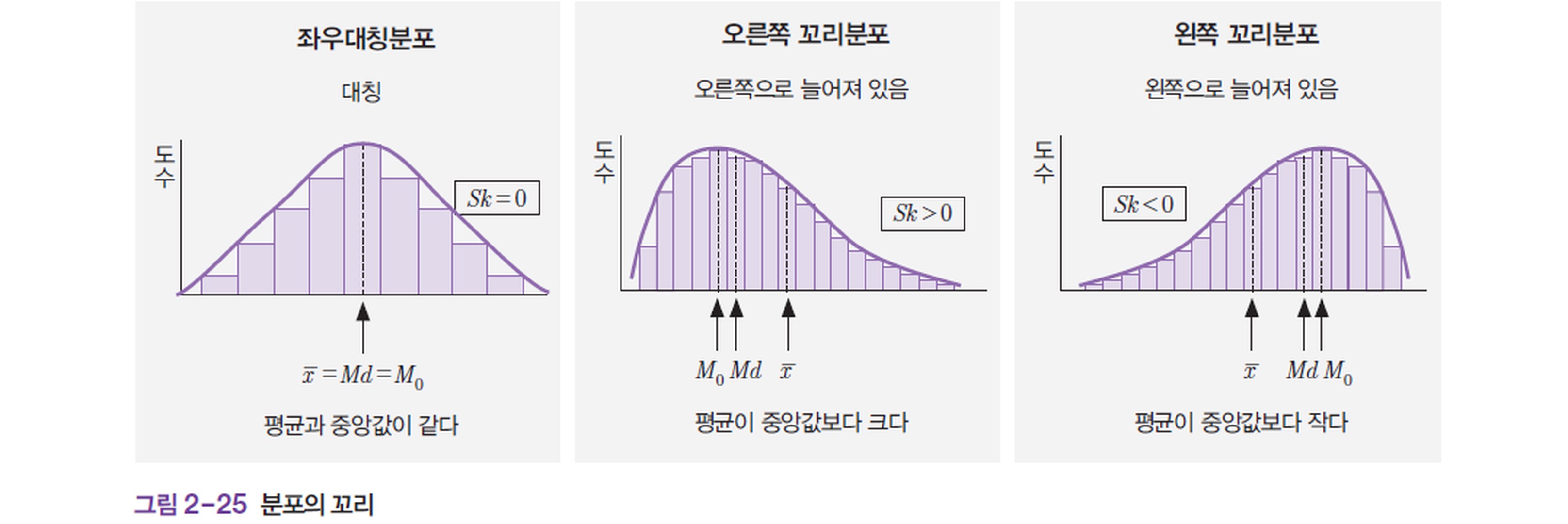
Figure 2-25 Tails of a distribution: a symmetric distribution (mean=median=mode), a right-tailed distribution (the mean is greater than the median), and a left-tailed distribution (the mean is less than the median)
### Supporting text from the original screen
49 / 77
The trap of the mean · 13/18
## 50\. R-Studio example 2: Ctrl+C / Ctrl+V the following code as is
```r
# 표준편차 곡선을 그리는 코드
curve(dnorm(x, mean = mean(student_data$salary), sd = sd(student_data$salary)),
from = min(student_data$salary),
to = max(student_data$salary),
xlab = "Salary",
ylab = "Density",
main = "연봉 분포와 표준편차 곡선",
col = "blue",
lwd = 2)
# 연봉 분포를 세로선으로 표시
abline(v = student_data$salary, col = "red", lty = 2)
```
### Supporting text from the original screen
50 / 77
The trap of the mean · 14/18
## 51\. R-Studio example 2: distribution of the average salary with a student earning 1 billion won mixed in
R graph ‘Salary distribution and standard deviation curve’: the normal distribution curve peaks on the left and falls off in a long slope to the right. Red dashed vertical lines are drawn at 5000 (14 people) and 100000 (1 person).
### Supporting text from the original screen
51 / 77
The trap of the mean · 15/18
## 52\. R-Studio example 2: Ctrl+C / Ctrl+V the following code as is
```r
# 정규분포를 따르는 salary 값을 생성하는 코드
set.seed(42) # 랜덤 시드를 설정하여 재현성을 보장합니다.
# 평균과 표준편차 지정
mean_salary <- mean(student_data$salary)
sd_salary <- sd(student_data$salary)
# 정규분포에 따르는 새로운 salary 값 생성
new_salary <- rnorm(n = nrow(student_data), mean = mean_salary, sd = sd_salary)
# 생성한 값들을 데이터프레임에 할당
student_data$salary <- new_salary
# 수정된 salary 값 출력
print(student_data$salary)
```
### Supporting text from the original screen
52 / 77
The trap of the mean · 16/18
## 53\. R-Studio example 2: normal distribution plot of students with evenly spread salaries
**R output**
```text
> print(student_data$salary)
[1] 44961.428 -2518.089 20240.472
[4] 26856.753 21249.588 8730.216
[7] 48409.297 9011.452 60843.036
[10] 9795.026 43340.343 67422.217
[13] -22733.884 4494.953 8063.108
```
### Supporting text from the original screen
53 / 77
The trap of the mean · 17/18
## 54\. Summary
| Mode | The value with the highest frequency among all the data |
| --- | --- |
| Median | The value located exactly in the middle when all the data are arranged in rank order from the lowest value to the highest |
| Mean | The value obtained by adding up all the data and then dividing the total by the number of data points |
Variance and standard deviation: a map that shows how the overall mean value is spread out when you line up the mean values horizontally from the low ones to the high ones
Of the three, the mean value is usually the most common, but there are cases, as with salaries, where the mean value does not apply (the mean value is not a cure-all!)
### Supporting text from the original screen
54 / 77
The trap of the mean · 18/18
## 55\. What is inferential statistics?
### Supporting text from the original screen
55 / 77
Inferential statistics · 1/23
## 56\. What is inferential statistics?
**Basic procedure of inferential statistics**
What is inferential statistics? An analytical method that uses sample data to make statistical inferences about a population
**Mean and variance**
| Sample mean | X̄ |
| --- | --- |
| Estimate of the population mean | μ = X̄ |
| Sample variance | S² |
| Estimate of the population variance | σ² = S²/n |
**Confidence interval**
### Supporting text from the original screen
56 / 77
Inferential statistics · 2/23
## 57\. Population and sample – how many strawberry chocolates are there in the whole box?
Candy-drawing simulator screen, with ‘Shall we grab just a tiny handful?’ and a fist with a few candies at the top right, the candy box (population) at the bottom left, and a photo of strawberry chocolates at the bottom right
### Supporting text from the original screen
57 / 77
Inferential statistics · 3/23
## 58\. Let us grab some candy with our fists.
**Population**
The method does not matter. What is the exact proportion of strawberry chocolate candies in the whole box?
**Shall we grab just a few?**
Sample 1
**OR · Shall we grab a fistful so full it bursts?**
Sample 2

Photos, from left: a box full of candy (population), a fist and only a few candies (Sample 1), and a fist and a big pile of bubble gum (Sample 2)
### Supporting text from the original screen
58 / 77
Inferential statistics · 4/23
## 59\. RQ. How many strawberry chocolate candies are there in total among all the original candies?
**Halloween candy box**
* Population: all the candies in the candy box
* Sample: the candies I drew from the box with my fist
### Supporting text from the original screen
59 / 77
Inferential statistics · 5/23
## 60\. RQ. How many strawberry chocolate candies are there in total among all the original candies?

**Population**

**I want to know how many “just strawberry chocolates” are in the box**
**Surely you are not going to tear open this whole box and count them one by one?**
### Supporting text from the original screen
60 / 77
Inferential statistics · 6/23
## 61\. Let us count only the candies in my hand (never mind the original box)
Candy-drawing simulator screen: at the top left, a slider for the number to draw and a table of counts for each kind of candy drawn; below, a bar chart by kind. At the bottom, photos of a fist with a few candies and of strawberry chocolates
### Supporting text from the original screen
61 / 77
Inferential statistics · 7/23
## 62\. Let us count only the candies in my hand (never mind the original box)
[https://posit.cloud/content/5906664](https://posit.cloud/content/5906664)
[https://posit.cloud/content/7862513](https://posit.cloud/content/7862513)
See the candy-drawing simulator R-Studio code.R
### Supporting text from the original screen
62 / 77
Inferential statistics · 8/23
## 63\. Candy-drawing simulator – try drawing on the web
Run it right in your browser: [https://claude.ai/artifact/B3vs3qRXH6HRe755AbKnyh](https://claude.ai/artifact/B3vs3qRXH6HRe755AbKnyh)
Candy-drawing simulator web screen: a sample size slider set to 100 and the \[Draw a sample\] · \[Draw 10 · 100 · 1000 times\] · \[Reset\] buttons; in the ‘Cumulative draws’ tab, a histogram of the strawberry chocolate proportions of 1,000 samples (a bell shape centered on 10%, with a dashed normal distribution curve); on the right, the mean · standard deviation of the sample proportions and the proportions for all 10 kinds of candy combined
### Supporting text from the original screen
63 / 77
Inferential statistics · 9/23
## 64\. Exercise. Let us count the number of candies and the strawberry chocolates with the candy-drawing simulator
| | Number of candies | Strawberry chocolates |
| --- | --- | --- |
| Sample 1 | | |
| Sample 2 | | |
| Sample 3 | | |
| Sample 4 | | |
| Sample 5 | | |
### Supporting text from the original screen
64 / 77
Inferential statistics · 10/23
## 65\. RQ. How many strawberry chocolate candies are there in total among all the original candies?

**Population**

**I want to know how many “just strawberry chocolates” are in the box**
Inferential statistics: estimating the proportion of strawberry chocolates in the original box from the proportion of strawberry chocolates in the sample
| | Number of candies | Strawberry chocolates |
| --- | --- | --- |
| Sample 1 | | |
| Sample 2 | | |
| Sample 3 | | |
| Sample 4 | | |
| Sample 5 | | |
### Supporting text from the original screen
65 / 77
Inferential statistics · 11/23
## 66\. RQ. How many strawberry chocolate candies are there in total among all the original candies?

**Population**
| | Number of candies | Strawberry chocolates |
| --- | --- | --- |
| Sample 1 | | |
| Sample 2 | | |
| Sample 3 | | |
| Sample 4 | | |
| Sample 5 | | |
**Inferential statistics:**
* Estimating the proportion of strawberry chocolates in the original box from the proportion of strawberry chocolates in the sample
* “My fist has this many strawberry chocolates, so judging from that, about how many would there be if I counted all the strawberry chocolates in the original box?” – Estimation
### Supporting text from the original screen
66 / 77
Inferential statistics · 12/23
## 67\. RQ. How many strawberry chocolate candies are there in total among all the original candies?
**Making the strawberry chocolate dataset (R-Studio code)**
```r
# 데이터 프레임 생성
candy_data <- data.frame(
Sample = c('샘플1', '샘플2', '샘플3', '샘플4', '샘플5'),
Total_Candies = c(100, 100, 100, 100, 100),
Strawberry_Chocolate = c(8, 7, 12, 9, 9)
)
# 데이터 확인
print(candy_data)
```
> Note: If the numbers you actually drew are different, change the Total and Strawberry numbers
### Supporting text from the original screen
67 / 77
Inferential statistics · 13/23
## 68\. Finding the descriptive statistics of the strawberry chocolates
```r
#최빈값:
freq <- table(candy_data$Strawberry_Chocolate)
maxfreq <- max(freq)
which(freq == maxfreq)
table(candy_data$Strawberry_Chocolate)
#중앙값:
median(candy_data$Strawberry_Chocolate)
#평균값:
mean(candy_data$Strawberry_Chocolate)
#분산:
var(candy_data$Strawberry_Chocolate)
#표준편차:
sd(candy_data$Strawberry_Chocolate)
```
> Note: candy\_data$Strawberry\_Chocolate has the structure ‘dataset$variable\_name’. For the rest of the descriptive statistics formulas, just use the formulas shown alongside as they are
### Supporting text from the original screen
68 / 77
Inferential statistics · 14/23
## 69\. Finding the descriptive statistics of the strawberry chocolates – R output
```text
> which(freq == maxfreq)
9
3
> table(candy_data$Strawberry_Chocolate)
7 8 9 12
1 1 2 1
> median(candy_data$Strawberry_Chocolate)
[1] 9
> mean(candy_data$Strawberry_Chocolate)
[1] 9
> var(candy_data$Strawberry_Chocolate)
[1] 3.5
> sd(candy_data$Strawberry_Chocolate)
[1] 1.870829
```
### Supporting text from the original screen
69 / 77
Inferential statistics · 15/23
## 70\. Inferential statistics: estimating the number of strawberry chocolates in the whole box
```r
# t.test를 사용하여 신뢰구간 계산
t.test(candy_data$Strawberry_Chocolate)$conf.int
```
**R output**
```text
> t.test(candy_data$Strawberry_Chocolate)$conf.int
[1] 6.677059 11.322941
attr(,"conf.level")
[1] 0.95
```
Note: candy\_data$Strawberry\_Chocolate has the structure ‘dataset$variable\_name’
For the rest of the descriptive statistics formulas, just use the formulas shown alongside as they are
### Supporting text from the original screen
70 / 77
Inferential statistics · 16/23
## 71\. Inferential statistics: estimating the number of strawberry chocolates in the whole box
```r
# t.test를 사용하여 신뢰구간 계산
t.test(candy_data$Strawberry_Chocolate)$conf.int
```
**t.test result**
```text
> t.test(candy_data$Strawberry_Chocolate)$conf.int
[1] 6.677059 11.322941
attr(,"conf.level")
[1] 0.95
```
**In other words, there is a 95% probability that the whole box contains between 6.68 and 11.32 strawberry chocolates**
### Supporting text from the original screen
71 / 77
Inferential statistics · 17/23
## 72\. The beginning of inferential statistics: sampling and estimation
**Characteristics of sample quantities**
Definition 3-1 Population, sample, parameter, statistic
* 1) Population: the entire group that is the object of interest
* 2) Sample: a subset of the population
* 3) Parameter: a characteristic value of the population (e.g., population mean, population proportion, population variance, etc.)
* 4) Statistic: a characteristic value of the sample (e.g., sample mean, sample proportion, sample variance, etc.)
### Supporting text from the original screen
72 / 77
Inferential statistics · 18/23
## 73\. Inferential statistics: estimating the population (the candy box) from candy sample statistics
**“We ‘estimate’ the population's parameters from the sample's statistics” = “I ‘estimate’ the distribution of candies in the candy box from the 100 candies in my fist”**
| Definition 3-1 · Population, sample, parameter, statistic | Candy example |
| --- | --- |
| Population: the entire group that is the object of interest | (the whole candy box) |
| Sample: a subset of the population | (the handful I drew with my fist, including strawberry chocolates) |
| Parameter: a characteristic value of the population (e.g., population mean, population proportion, population variance, etc.) | (the mean, frequency, etc. of each candy in the whole candy box) |
| Statistic: a characteristic value of the sample (e.g., sample mean, sample proportion, sample variance, etc.) | (the mean, frequency, etc. of each candy in my fist) |
### Supporting text from the original screen
73 / 77
Inferential statistics · 19/23
## 74\. Premise 1 of inferential statistics: the population cannot be known ‘exactly’

**“We ‘estimate’ the population's parameters from the sample's statistics” = “I ‘estimate’ the distribution of candies in the candy box from the 100 candies in my fist”**
“I ‘estimate’ the distribution of candies in the candy box from the 100 candies in my fist”
\= in other words, it is impossible to know ‘exactly how many’ strawberry chocolates are in the candy box
(one of the most important premises of statistics)
### Supporting text from the original screen
74 / 77
Inferential statistics · 20/23
## 75\. Premise 2 of inferential statistics: there is always a chance of being wrong
```r
# t.test를 사용하여 신뢰구간 계산
t.test(candy_data$Strawberry_Chocolate)$conf.int
```
**t.test result**
```text
> t.test(candy_data$Strawberry_Chocolate)$conf.int
[1] 6.677059 11.322941
attr(,"conf.level")
[1] 0.95
```
**In other words, there is a 95% probability that the whole box contains between 6.68 and 11.32 strawberry chocolates**
> → There is a 5% chance that I could be wrong (there is no such thing as a zero chance of being wrong)
### Supporting text from the original screen
75 / 77
Inferential statistics · 21/23
## 76\. Premise 3 of inferential statistics: a ‘standard error’ exists (a number that shows how wrong I am)
**“We ‘estimate’ the population's parameters from the sample's statistics” = “I ‘estimate’ the distribution of candies in the candy box from the 100 candies in my fist”**
(e.g., the number of mint candies in the population estimated from the 100 candies in my fist = 3.4 billion)
* Huh, the actual number is 3.59 billion, but it does not match the 3.4 billion I predicted?
* Standard error: the degree of “how wrong I was” expressed as a number (the degree of difference between the population parameter and the parameter estimated from the sample's descriptive statistics)
### Supporting text from the original screen
76 / 77
Inferential statistics · 22/23
## 77\. Summary of the basics of inferential statistics
* It is impossible to know perfectly a specific parameter of the population (e.g., the total number of strawberry chocolates in the box)
* Searching through the entire population (inside the box) is a brute-force and inefficient method
* I count only the candies in my palm, then “estimate” the original box from the “pattern” of the candies in my palm
* We cannot know the perfect answer because we “estimate” (we guess using probability)
* “(Since I cannot guess the population perfectly) how wrong I am” = the standard error.

**Population**

**I want to know how many “just strawberry chocolates” are in the box**
Surely you are not going to tear open this whole box and count them one by one?
### Supporting text from the original screen
77 / 77
Inferential statistics · 23/23