Report variance assumptions and pairwise corrections together
Present group distributions with multiplicity-corrected contrast intervals. Keep the overall F test separate from each pairwise conclusion.
Classical F + Tukey · 944 respondents · ANES96
01 · The presentation slide
CMDS · SVG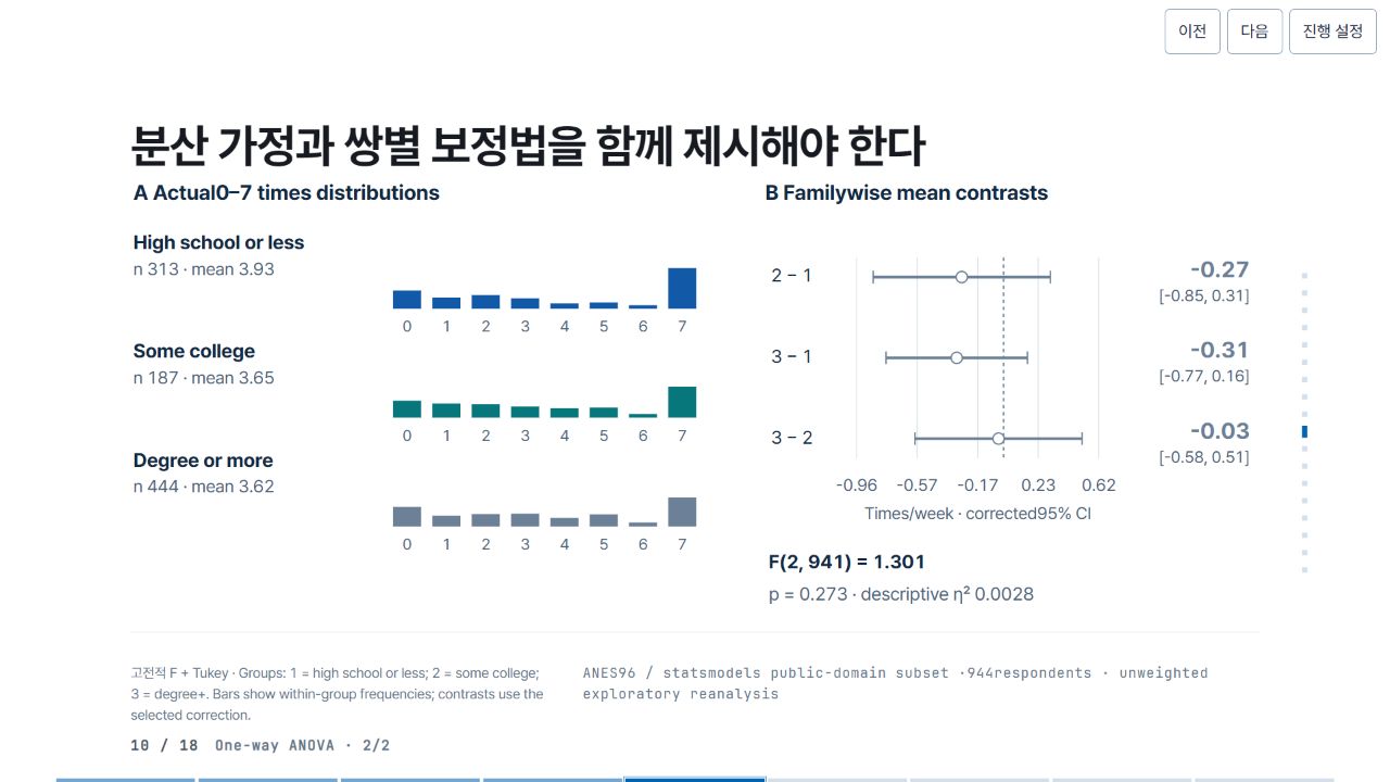
02 · Pele relationship map and source
Pele 1.6.0 · Mermaid flowchartThis companion diagram explains variables, design and tests. It is distinct from the statistical figure in the standalone presentation.

Pele map source
flowchart LR
 E["Education3groups"] --> Y["TV-news distribution"]
 Y --> F["Overall F"]
 Y --> P["Corrected pair contrasts"]
 P --> C["Uncertainty retained"]
03 · Precision SVG construction code
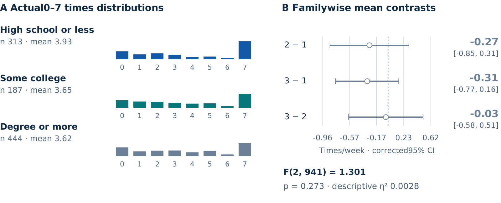
JavaScript → SVGThis actual production branch takes computed estimates and places axes, lines, intervals and labels. Shared helpers and the complete file are available below.
SVG construction branch · JavaScript
if (v.kind === "anova") {
  a.push(
    T(0, 35, "A  Actual0–7 times distributions", 30, C.ink, 700),
    T(900, 35, "B  Familywise mean contrasts", 30, C.ink, 700),
  );
  const cols = [C.blue, C.teal, C.slate];
  v.groups.forEach((g, i) => {
    let yy = 105 + i * 155;
    a.push(
      T(0, yy, g.label, 28, C.ink, 650),
      T(0, yy + 37, "n " + g.n + " · mean " + fmt(g.mean, 2), 25, C.muted),
    );
    for (let d = 0; d < 8; d++) {
      let n = g.hist.find((a) => a[0] === d)?.[1] || 0,
        h = (n / g.n) * 155;
      a.push(
        G(
          [
            R(370 + d * 56, yy + 85 - h, 40, h, cols[i]),
            T(390 + d * 56, yy + 118, String(d), 22, C.muted, 400, "middle"),
          ],
          g.key,
        ),
      );
    }
  });
  a.push(
    ...forest(v.contrasts, {
      x: 900,
      y: 50,
      w: 700,
      labelW: 130,
      rowH: 115,
      title: "",
      unit: "Times/week · corrected95% CI",
    }),
    T(
      905,
      560,
      "F(" + v.df.map((x) => fmt(x, 1)).join(", ") + ") = " + fmt(v.F, 3),
      27,
      C.ink,
      650,
    ),
    T(
      905,
      605,
      pv(v.p) + " · descriptive η² " + fmt(v.eta2Descriptive, 4),
      26,
      C.muted,
    ),
  );
  note =
    "Groups: 1 = high school or less; 2 = some college; 3 = degree+. Bars show within-group frequencies; contrasts use the selected correction.";
  source =
    'flowchart LR\n E["Education3groups"] --> Y["TV-news distribution"]\n Y --> F["Overall F"]\n Y --> P["Corrected pair contrasts"]\n P --> C["Uncertainty retained"]';
  map = { E: v.groups[0].key, Y: v.groups[1].key, F: v.key, P: v.key, C: v.key };
}
This is preserved reference code, not an executable editor.
04 · What to change when reusing it
DATA · DESIGN · INFERENCE- Data
- Inspect the condition data first. Replace sample, units, coefficients and confidence intervals together. Do not combine different samples or measurement levels on one scale.
- Graphic
- Fit axis ranges, label widths, type and colors to the target region. Preserve whether intervals include zero and recheck legibility at the final size.
- Interpretation
- Diagram arrows and model paths are not causal evidence. Distinguish mean-response from prediction intervals, and pointwise from simultaneous intervals.