The association remains visible at the original seven levels
Compare observed and expected counts with standardized residuals. Combining categories changes the question and degrees of freedom.
Original seven levels · 944 respondents · ANES96
01 · The presentation slide
CMDS · SVG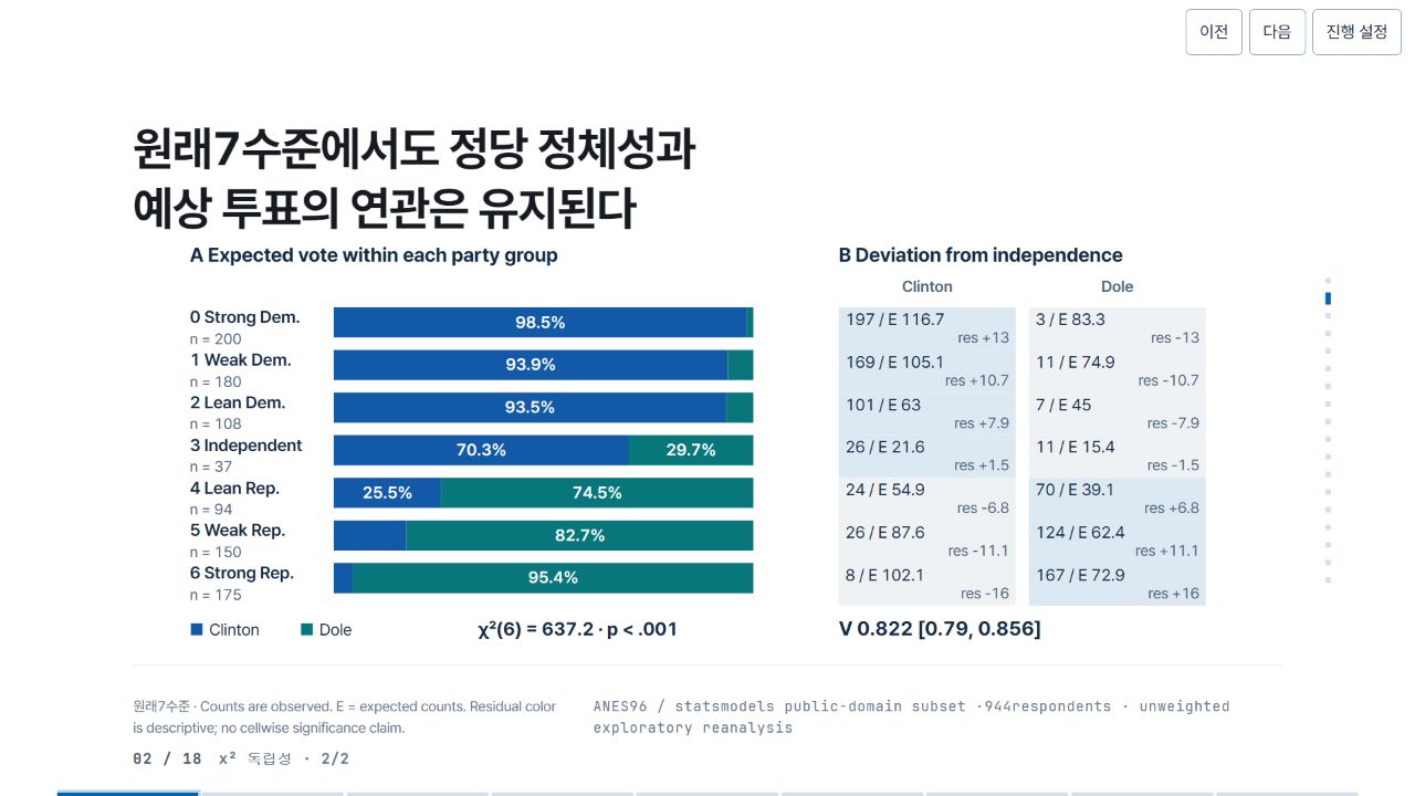
02 · Pele relationship map and source
Pele 1.6.0 · Mermaid flowchartThis companion diagram explains variables, design and tests. It is distinct from the statistical figure in the standalone presentation.

Pele map source
flowchart LR
 P["Party identification"] --- V["Expected vote"]
 P --> C["Observed × expected counts"]
 V --> C
 C --> R["Residuals + Cramer V"]
03 · Precision SVG construction code
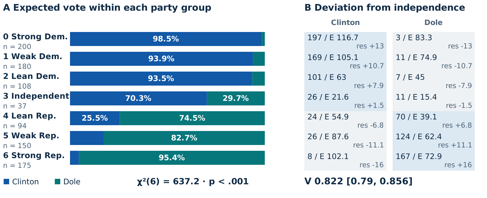
JavaScript → SVGThis actual production branch takes computed estimates and places axes, lines, intervals and labels. Shared helpers and the complete file are available below.
SVG construction branch · JavaScript
if (v.kind === "chi") {
  a.push(
    T(10, 35, "A  Expected vote within each party group", 30, C.ink, 700),
    T(1000, 35, "B  Deviation from independence", 30, C.ink, 700),
    T(1135, 82, "Clinton", 24, C.muted, 600, "middle"),
    T(1425, 82, "Dole", 24, C.muted, 600, "middle"),
  );
  let rh = v.rows.length > 3 ? 65 : 145,
    top = 105;
  v.rows.forEach((r, i) => {
    let yy = top + i * rh,
      cs = v.cells.filter((c) => c.i === i);
    a.push(
      T(
        10,
        yy + 24,
        v.rows.length > 3
          ? [
              "0 Strong Dem.",
              "1 Weak Dem.",
              "2 Lean Dem.",
              "3 Independent",
              "4 Lean Rep.",
              "5 Weak Rep.",
              "6 Strong Rep.",
            ][+r]
          : r,
        26,
        C.ink,
        600,
      ),
      T(10, yy + 56, "n = " + cs.reduce((n, c) => n + c.obs, 0), 23, C.muted),
    );
    let xx = 230;
    for (const c of cs) {
      let width = c.pct * 6.4,
        col = c.j === 0 ? C.blue : C.teal;
      a.push(
        G(
          [
            R(xx, yy, Math.max(1, width), 46, col),
            ...(width > 112
              ? [
                  T(
                    xx + width / 2,
                    yy + 31,
                    fmt(c.pct, 1) + "%",
                    25,
                    "#FFFFFF",
                    600,
                    "middle",
                  ),
                ]
              : []),
          ],
          c.key,
        ),
      );
      xx += width;
      let cx = 1000 + c.j * 290;
      let strength = Math.min(1, Math.abs(c.residual) / 15),
        fill = c.residual > 0 ? "#DCE9F3" : "#EFF2F4";
      a.push(
        G(
          [
            R(cx, yy, 270, 65, fill),
            T(cx + 10, yy + 27, c.obs + " / E " + fmt(c.expected, 1), 25),
            T(
              cx + 260,
              yy + 54,
              "res " + signed(c.residual, 1),
              23,
              C.muted,
              400,
              "end",
            ),
          ],
          c.key,
        ),
      );
    }
  });
  a.push(
    R(12, 587, 18, 18, C.blue),
    T(40, 605, "Clinton", 25),
    R(180, 587, 18, 18, C.teal),
    T(208, 605, "Dole", 25),
    T(
      450,
      605,
      "χ²(" + v.df + ") = " + fmt(v.stat, 1) + " · " + pv(v.p),
      28,
      C.ink,
      650,
    ),
    G(
      [
        T(
          1000,
          605,
          "V " +
            fmt(v.effect, 3) +
            "  [" +
            v.effectCI.map((x) => fmt(x, 3)).join(", ") +
            "]",
          30,
          C.ink,
          700,
        ),
      ],
      v.key,
    ),
  );
  note =
    "Counts are observed. E = expected counts. Residual color is descriptive; no cellwise significance claim.";
  source =
    'flowchart LR\n P["Party identification"] --- V["Expected vote"]\n P --> C["Observed × expected counts"]\n V --> C\n C --> R["Residuals + Cramer V"]';
  map = { P: v.key, V: v.cells[0].key, C: v.cells[1].key, R: v.key };
}
This is preserved reference code, not an executable editor.
04 · What to change when reusing it
DATA · DESIGN · INFERENCE- Data
- Inspect the condition data first. Replace sample, units, coefficients and confidence intervals together. Do not combine different samples or measurement levels on one scale.
- Graphic
- Fit axis ranges, label widths, type and colors to the target region. Preserve whether intervals include zero and recheck legibility at the final size.
- Interpretation
- Diagram arrows and model paths are not causal evidence. Distinguish mean-response from prediction intervals, and pointwise from simultaneous intervals.