Age remains associated with news use after adjustment
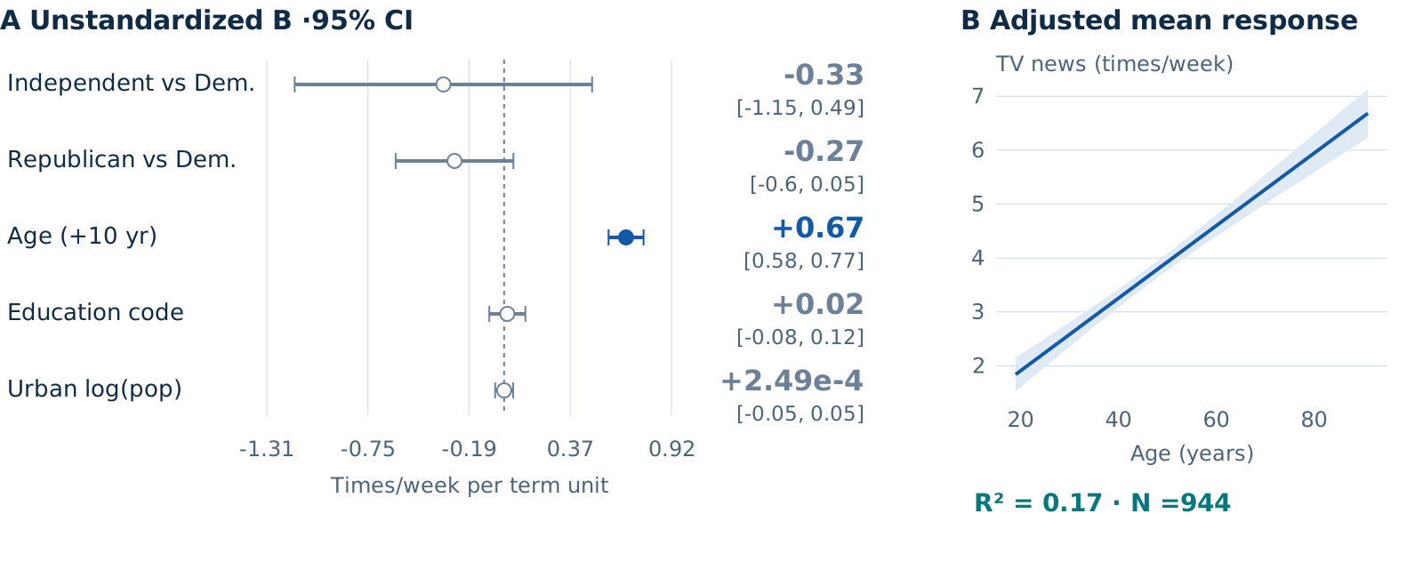
Link a coefficient forest to the adjusted mean response. OLS and HC3 intervals may differ while data and coefficients remain the same.
Classical standard errors · 944 respondents · ANES96
01 · The presentation slide
CMDS · SVG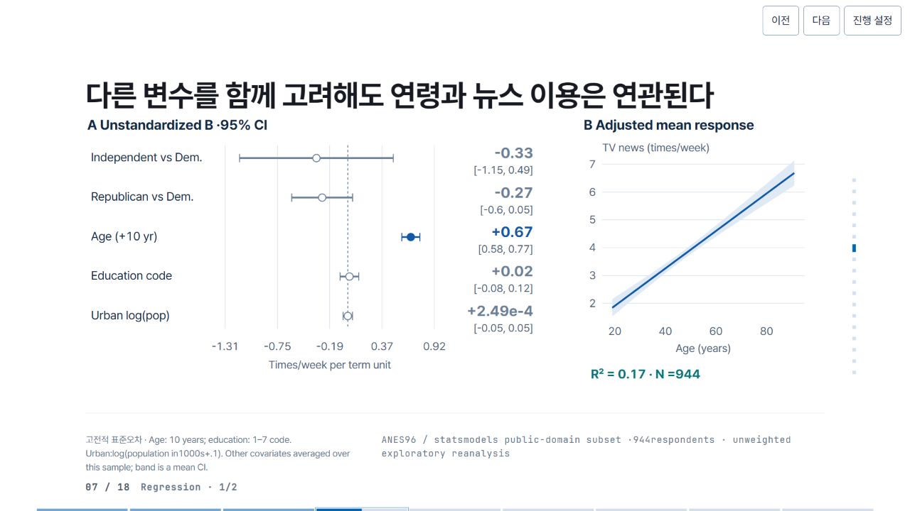
02 · Pele relationship map and source
Pele 1.6.0 · Mermaid flowchartThis companion diagram explains variables, design and tests. It is distinct from the statistical figure in the standalone presentation.

Pele map source
flowchart LR
 A["Age"] --> Y["TV news"]
 E["Education code"] --> Y
 U["Urban scale"] --> Y
 P["Party group"] --> Y
 Y --> R["Conditional association"]
03 · Precision SVG construction code
JavaScript → SVGThis actual production branch takes computed estimates and places axes, lines, intervals and labels. Shared helpers and the complete file are available below.
SVG construction branch · JavaScript
if (v.kind === "regression") {
  let rows = v.coef
    .filter((x) => x.term !== "Intercept")
    .map((x) => ({ ...x, label: short[x.term] || x.term }));
  a.push(
    ...forest(rows, {
      x: 0,
      y: 0,
      w: 980,
      labelW: 300,
      rowH: 86,
      title: "A  Unstandardized B ·95% CI",
      unit: "Times/week per term unit",
    }),
  );
  a.push(T(1080, 33, "B  Adjusted mean response", 30, C.ink, 700));
  let pp = plotFrame({
    x: 1120,
    y: 100,
    w: 440,
    h: 340,
    xRange: [15, 95],
    yRange: [
      Math.min(2, ...v.predictions.map((p) => p.lo)),
      Math.max(7, ...v.predictions.map((p) => p.hi)),
    ],
    xTicks: [20, 40, 60, 80],
    yTicks: [2, 3, 4, 5, 6, 7],
    xLabel: "Age (years)",
    yLabel: "TV news (times/week)",
  });
  a.push(
    ...pp.a,
    G(curve(v.predictions, pp.X, pp.Y), v.key),
    T(1095, 575, "R² = " + fmt(v.r2, 3) + " · N =944", 28, C.teal, 700),
  );
  note =
    "Age: 10 years; education: 1–7 code. Urban:log(population in1000s+.1). Other covariates averaged over this sample; band is a mean CI.";
  source =
    'flowchart LR\n A["Age"] --> Y["TV news"]\n E["Education code"] --> Y\n U["Urban scale"] --> Y\n P["Party group"] --> Y\n Y --> R["Conditional association"]';
  map = {
    A: v.key,
    E: rows.find((x) => x.term === "educ")?.key,
    U: rows.find((x) => x.term === "logpopul")?.key,
    P: rows.find((x) => x.term.includes("Independent"))?.key,
    Y: v.key,
    R: v.key,
  };
}
This is preserved reference code, not an executable editor.
04 · What to change when reusing it
DATA · DESIGN · INFERENCE- Data
- Inspect the condition data first. Replace sample, units, coefficients and confidence intervals together. Do not combine different samples or measurement levels on one scale.
- Graphic
- Fit axis ranges, label widths, type and colors to the target region. Preserve whether intervals include zero and recheck legibility at the final size.
- Interpretation
- Diagram arrows and model paths are not causal evidence. Distinguish mean-response from prediction intervals, and pointwise from simultaneous intervals.