강건한 오차에서도 상호작용 구간은0을 포함한다
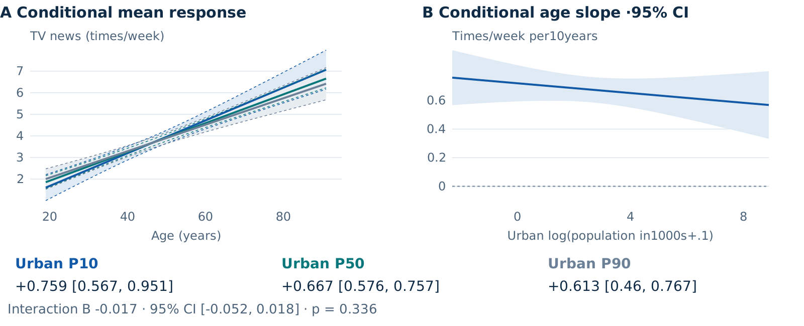
관측된 조절변수 범위에서 조건부 기울기를 보여줍니다. P10·P50·P90 예측선과 점별 구간, 전체 상호작용 검정을 구분합니다.
HC3 조건부 효과 · 944 respondents · ANES96
01 · 실제 발표 장표
CMDS · SVG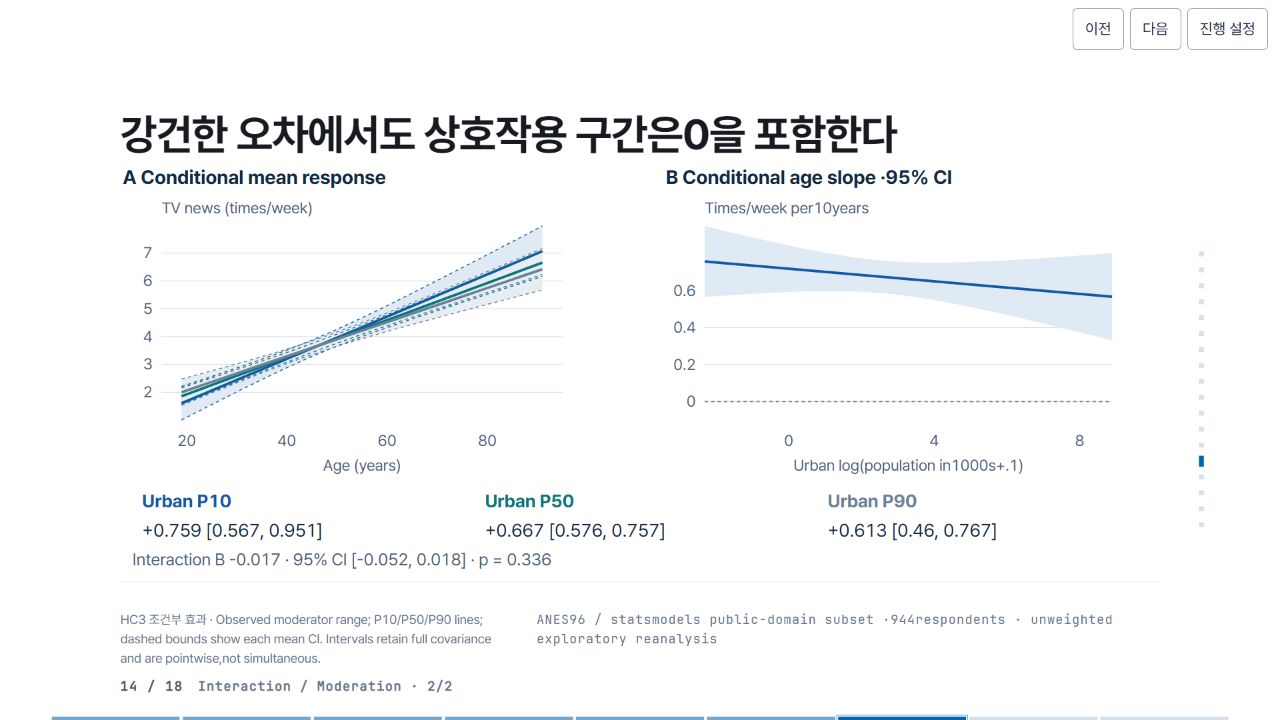
02 · Pele 관계도와 원문
Pele 1.6.0 · Mermaid flowchart이 관계도는 분석의 변수·설계·검정 관계를 설명하는 보조 도식입니다. 단독 HTML 발표 장표의 통계 그림과 구분합니다.

Pele 관계도 원문
flowchart LR
 A["Age"] --> N["TV news"]
 U["Urban scale"] --> N
 I["Age × urban"] --> N
 N --> S["Conditional slopes + CI"]
03 · 정밀 SVG 제작 코드
JavaScript → SVG공개된 추정치를 받아 축·선·구간·라벨을 직접 배치하는 실제 제작 분기입니다. 생략한 공용 함수와 전체 파일도 확인할 수 있습니다.
SVG 제작 분기 · JavaScript
if (v.kind === "moderation") {
  a.push(
    T(0, 35, "A  Conditional mean response", 30, C.ink, 700),
    T(840, 35, "B  Conditional age slope ·95% CI", 30, C.ink, 700),
  );
  let p1 = plotFrame({
      x: 60,
      y: 100,
      w: 620,
      h: 300,
      xRange: [15, 95],
      yRange: [
        Math.min(2, ...v.curves.flat().map((p) => p.lo)),
        Math.max(7, ...v.curves.flat().map((p) => p.hi)),
      ],
      xTicks: [20, 40, 60, 80],
      yTicks: [2, 3, 4, 5, 6, 7],
      xLabel: "Age (years)",
      yLabel: "TV news (times/week)",
    }),
    p2 = plotFrame({
      x: 900,
      y: 100,
      w: 630,
      h: 300,
      xRange: [Math.min(...v.jn.map((x) => x.x)), Math.max(...v.jn.map((x) => x.x))],
      yRange: [
        Math.min(-0.1, ...v.jn.map((x) => x.lo)),
        Math.max(0.7, ...v.jn.map((x) => x.hi)),
      ],
      xTicks: [0, 4, 8],
      yTicks: [0, 0.2, 0.4, 0.6],
      xLabel: "Urban log(population in1000s+.1)",
      yLabel: "Times/week per10years",
    });
  a.push(...p1.a, ...p2.a);
  v.curves.forEach((c, i) =>
    a.push(
      G(
        curve(c, p1.X, p1.Y, [C.blue, C.teal, C.slate][i], true).slice(0, 1),
        v.slopes[i].key,
      ),
    ),
  );
  v.curves.forEach((c, i) => {
    let col = [C.blue, C.teal, C.slate][i];
    for (const edge of ["lo", "hi"])
      a.push(
        G(
          [
            D(
              c
                .map((p, j) => (j ? "L" : "M") + p1.X(p.x) + " " + p1.Y(p[edge]))
                .join(" "),
              col,
              1.5,
              "none",
              { "stroke-dasharray": "5 5" },
            ),
          ],
          v.slopes[i].key,
        ),
      );
    a.push(G(curve(c, p1.X, p1.Y, col, false), v.slopes[i].key));
  });
  a.push(
    G(curve(v.jn, p2.X, p2.Y), v.key),
    L(900, p2.Y(0), 1530, p2.Y(0), C.slate, 2, "5 5"),
  );
  v.slopes.forEach((s, i) => {
    let xx = 30 + i * 530;
    a.push(
      G(
        [
          T(xx, 535, "Urban " + s.label, 28, [C.blue, C.teal, C.slate][i], 700),
          T(
            xx,
            580,
            signed(s.b, 3) + " [" + fmt(s.lo, 3) + ", " + fmt(s.hi, 3) + "]",
            28,
          ),
        ],
        s.key,
      ),
    );
  });
  a.push(
    G(
      [
        T(
          15,
          625,
          "Interaction B " +
            signed(v.interaction.value, 3) +
            " · 95% CI [" +
            v.interaction.ci.map((x) => fmt(x, 3)).join(", ") +
            "] · " +
            pv(v.interaction.p),
          26,
          C.muted,
        ),
      ],
      v.key,
    ),
  );
  note =
    "Observed moderator range; P10/P50/P90 lines; dashed bounds show each mean CI. Intervals retain full covariance and are pointwise,not simultaneous.";
  source =
    'flowchart LR\n A["Age"] --> N["TV news"]\n U["Urban scale"] --> N\n I["Age × urban"] --> N\n N --> S["Conditional slopes + CI"]';
  map = {
    A: v.slopes[0].key,
    U: v.slopes[2].key,
    I: v.key,
    N: v.key,
    S: v.slopes[1].key,
  };
}
이 소스는 실행 가능한 편집기가 아니라 원문을 보존한 참고 코드입니다.
04 · 재사용할 때 바꿀 것
DATA · DESIGN · INFERENCE- 데이터
- 해당 조건의 데이터 파일을 먼저 확인하고, 표본·단위·계수·신뢰구간을 함께 교체합니다. 표본이나 측정 수준이 다른 분석을 같은 척도로 합치지 않습니다.
- 그림
- 축 범위·라벨 폭·서체·색상은 실제 삽입 영역에 맞춥니다. 신뢰구간이 0을 포함하는지에 따라 의미를 보존하고, 화면을 줄인 뒤 다시 읽어 봅니다.
- 해석
- 관계도의 화살표와 통계 모형의 경로는 인과의 증거가 아닙니다. 평균 반응의 구간과 개별 예측구간, 점별 구간과 동시 구간을 구분합니다.